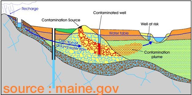
Course Introduction & Water Cycle
Contents
2. Course Introduction & Water Cycle#
(The contents presented in this section were re-developed principally by Dr. P. K. Yadav. The original contents were developed by Prof. Rudolf Liedl)
2.1. Contents of “Groundwater Module ”#
The entire contents of this interactive book can be listed with the following points:
general overview
types of aquifers, properties of aquifers
forces and pressure in the subsurface
laws of groundwater flow and some applications (e.g. groundwater wells)
quantification of aquifer parameter values via pumping tests
transport of chemicals (solutes) in groundwater
retardation and degradation of chemicals in groundwater
groundwater modelling
2.2. Suggested Literature:#
Brassington R. (1988): Field hydrogeology, Wiley & Sons.
Domenico P. A., Schwartz F. W. (1990): Physical and chemical hydrogeology, Wiley & Sons.
Fetter C. W. (2001): Applied hydrogeology, Prentice Hall.
Freeze R. A., Cherry J. A. (1979): Groundwater, Prentice Hall.
Heath R. C. (1987): Basic groundwater hydrology, USGS Water Supply Paper 2220.
Price M. (1996): Introducing groundwater, Chapman and Hall.
Additional literature details are provided in the text when used.
2.3. What is Hydrogeology?#
Hydrogeology is the study of the laws governing the movement of subterranean water, the mechanical, chemical, and thermal interaction of this water with the porous solid, and the transport of energy and chemical constituents by the flow. (Domenico and Schwartz, 1990)
The dominant reliance of groundwater for the drinking globally has made hydrogeology a very important academic course. Also, it is a very important research field. Therefore, several techniques and methods are now available to explore and understand Hydrogeological Process. The methods and techniques can be broadly categorized to:
Field works
Laboratory experiments
Computer modeling
Computer modelling is often the most economical method but its usefullness rely of data obtained from Field works and Laboratory experiments. Thus, the sequence of techniques/methods to be adopted depends on the available site information.
2.4. Example: Groundwater Extraction Well#
Groundwater is extracted using a groundwater well applying hydrogeological methods and techniques. The procedure followed can be summarized in the following steps:
The appropriate extraction location is identified
Drilling machine are used to obtain sub-surface structure, i.e. or well logs are obtained. The process is also called well logging.
Well logs are studied in detail to identify the characteristics of the subsurface- e.g., how thick is the aquifer or identify environmental consequence of water extraction.
The construction of well begins
Groundwater extraction using well is a challenge when aquifers are located very deep from the surface, e.g., in deserts.
2.5. Groundwater and Global Water Cycle#
Water bodies that exist on earth is connected, and they function as a cycle, called Global Water Cycle. It is estimated that over 57, 700 Km\(^3\) of water actively participates in the cycle each year. Precipitation and evaporation are the two main components of the cycle in which temperature plays the critical role. In the cycle, Groundwater receives water from precipitation, It then contributes to evaporation through subsurface flow or through mostly human intervention (e.g., use for drinking water).
The water cycle provides an approach to judge the sustainability of groundwater extraction. The sustainability of extraction can be obtained if extraction rate approximately equals the replenishing rate. Often the replenishing rate of groundwater is much slower and this has led to groundwater stress in many parts of the world.
2.6. The Hydrological Balance#
Since groundwater is part of the global water cycle, the balance of the cycle becomes an important topic. In general:
The hydrological balance provides a relationship between various flow rates for a certain area. It is based on the conservation of water volume.
expressed in words: inflow equals outflow plus change in storage
expressed by a formula:
The change in storage can be interpreted in the following way:
change in storage \(\Delta S > 0\) : Water volume is increasing with time in the investigation area.
change in storage \(\Delta S < 0\):Water volume is decreasing with time in the investigation area.
change in storage \(\Delta S = 0\): Water volume does not change with time in the investigation area (steady-state or stationary situation, i.e. inflow equals outflow).
2.7. Water Volume#
So how much water do we have?
It is estimated* that the total volume of water on Earth amounts to ca. 1 358 710 150 km\(^3\) (\(\approx\) 1018 m\(^3\)).
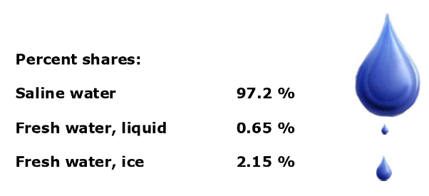
The total volume of fresh water on Earth amounts to ca. \(38\times 10^6\) km\(^3\) (\(\approx\) 1016 m\(^3\)).
*Gleick P. (1996): Water re-sources, in: Schneider S. H. (ed.), Encyclopedia of climate and weather 2, Oxford Univ. Press.
2.8. Volume of Available Fresh Water#
Fresh water are water with low concentrations of dissolved salts and other total dissolved solids, i.e., sea/ocean water or brackish water are not fresh water. Human activities (drinking water) are directly dependent on fresh activities.
So how much fresh water do we have?
It is estimated* that the total volume of available fresh water (liquid) on Earth amounts to ca. 8 831 600 km\(^3\) (\(\approx\) 1016 m\(^3\)).
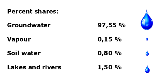
*Gleick P. (1996): Water re-sources, in: Schneider S. H. (ed.), Encyclopedia of climate and weather 2, Oxford Univ. Press.
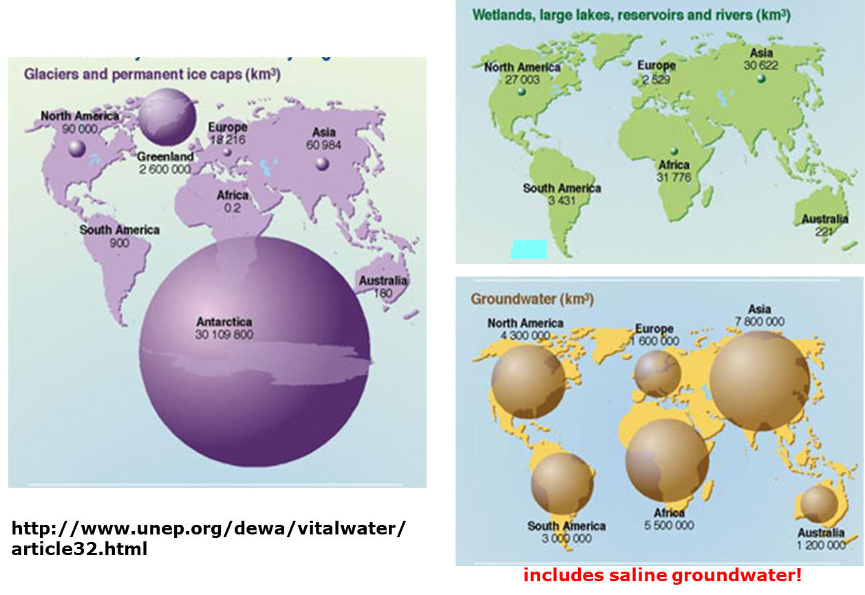
2.9. Continental distribution of fresh water components#
2.10. Volume and Mass Budget#
Very basics of volume and mass budget - let us start with budget.
Budget = quantitative comparison of growth (or production) and loss in a system
Budgets can be put together for various quantities:
energy
mass \(\leftarrow\) needed to quantify transport of solutes in groundwater
volume \(\leftarrow\) needed to quantify groundwater flow
momentum
electric charge
number of inhabitants
animal population
money (bank account!)
and many others
In this course we focus on Mass Budget and Volume Budget.
2.11. Volume Budget#
As discussed in the last topic a budget represents the change (e.g., growth and loss). Thus, it is more suitable to quantify the volume budget in terms of a change, representing two different states (e.g., time \((t)\)). More formally, the volume budget (\(\Delta V\)) can be obtained from:
with,
\(\Delta t\) = time interval [T]
\(\Delta V\) = change of volume in the system [L\(^3\)]
\(Q_{in}\) = volumetric rate of flow into the system [L\(^3\)/T]
\(Q_{out} =\) volumetric rate of flow out of the system [L\(^3\)/T]
The following points have to be considered when using the above equation:
Inflow and outflow may each consist of several individual components.
\(\Delta V = 0\) (no change in volume) is tantamount to steady-state or stationary (= time-independent) conditions.
For steady-state conditions we have: \(Q_{in} = Q_{out}\)
2.11.1. Water Budget for a Catchment#
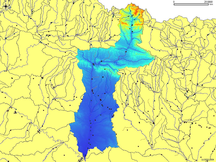
The equation provided for volume budget looks simple but in practice it is very complicated as several inflow and outflow components must be considered. Quantifying these components can be a challenging task.
For quantifying water budget of a catchment, one has to consider the following components:
To be considered:
precipitation
evapotranspiration
surface runoff
subsurface runoff
Among the above components, quantification of evapotranspiration and subsurface runoff have very high level of uncertainties.
2.12. Example: Estimation of Subsurface Runoff#
Most numbers used in the example do not refer to the catchment shown before!
To calculate the following four-steps are to be followed:
Step 1: determine rate of inflow in m³/a
step 2: determine rate of outflow due to evapotranspiration (ET.A) in m³/a
Step 3: express rate of outflow due to surface runoff in m³/a
step 4: determine rate of outflow due to subsurface runoff
An Example:
For given data, determine the rate of outflow Qout,sub due to subsurface runoff for steady-state conditions
A = 4500 # km², catchment area
P = 550 # mm/a, precipitation
ET = 200 # mm/a, evapotranspiration
Qout_surf = 40 # m³/s, surface runoff
Delta_V = 0 # m³, change in volume = 0 Steady-state conditions
#Volume budget in this example: P·A = ET·A + Qout,surf + Qout,sub
#Step 1
Qin = P*A*10**3 #m³/a, 10^3 for unit conversion
#step 2:
ET_A = ET*A*10**3 #m³/a, 10^3 for unit conversion
#Step 3:
Qout_surf = Qout_surf *365*24*3600 # m³/a
# step 4:
Qout_sub = Qin - ET_A - Qout_surf # m³/a
print("The rate of inflow, Qin is {0:1.1E}".format(Qin),"m\u00b3/a \n"); print("The outflow rate due to Evapotranspiration is {0:1.1E}".format(ET_A),"m\u00b3/a \n")
print("The surface outflow rate, Q_out_surf in m\u00b3/a is {0:1.1E}".format(Qout_surf),"m\u00b3/a \n");print("The subsurface outflow rate, Qout_surf in m\u00b3/a is {0:1.1E}".format(Qout_sub),"m\u00b3/a \n")
The rate of inflow, Qin is 2.5E+09 m³/a
The outflow rate due to Evapotranspiration is 9.0E+08 m³/a
The surface outflow rate, Q_out_surf in m³/a is 1.3E+09 m³/a
The subsurface outflow rate, Qout_surf in m³/a is 3.1E+08 m³/a
2.13. Mass Budget#
The mass budget is quantified similar to the volume budget. Mathematically, the mass budget is:
with
\(\Delta t\) = time interval [T]
\(\Delta M\) = change of mass in the system [M]
\(J_{in}\) = rate of mass flow into the system [M/T]
\(J_{out}\) = rate of mass flow out of the system [M/T]
Similar to volume budget, the following points have to be considered in quantifying mass budget:
Inflow and outflow may each consist of several individual components.
\(\Delta M\) = 0 (no change in mass) is tantamount to steady-state or stationary
(= time-independent) conditions.For steady-state conditions we have: \(J_{in}\)= \(J_{out}\)
2.14. Example of Mass Budget: Radioactive Decay#
Consider a decay chain comprising of the three chemicals: A, B and C
decay chain: A \(\rightarrow\) B \(\rightarrow\) C
30% of \(\text{A}\) and 20% of \(\text{B}\) decay each year.
decay rate of \(\text{A}\) = production rate of \(\text{B}\) = \(0.3 \cdot a^{-1}\cdot M_A\)
decay rate of \(\text{B}\) = production rate of \(\text{C}\) = \(0.2\cdot a^{-1}\cdot M_B\)
mass budgets for \(\text{A}\), \(\text{B}\) and \(\text{C}\):
\begin{equation*} \begin{split} \Delta M_A &= 0.3 \text{ a \(^{-1}\) } \cdot M_A \cdot \Delta t \ \Delta M_B &= 0.3 \text{a\(^{-1}\)} \cdot M_A \cdot \Delta t - 0.2 \text{ a\(^{-1}\)} \cdot M_B \cdot \Delta t \ \Delta M_C &= 0.2 \text{a\(^{-1}\)} \cdot M_B \cdot \Delta t \end{split} \end{equation*}
Similar equations hold for quantitative descriptions of some chemical reactions which correspond to the type A \(\rightarrow\) B \(\rightarrow\) C
def mass_bal(n_simulation, MA, MB, MC, R_A, R_B):
A = np.zeros(n_simulation)
B = np.zeros(n_simulation)
C = np.zeros(n_simulation)
time = np.arange(n_simulation)
for i in range(0,n_simulation-1):
A[0] = MA
B[0] = MB
C[0] = MC
A[i+1] = A[i]-R_A*A[i]
B[i+1] = B[i]+R_A*A[i]-R_B*B[i]
C[i+1] = C[i]+R_B*B[i]
summ = A[i]+B[i]+C[i]
d = {"Mass_A": A, "Mass_B": B, "Mass_C": C, "Total Mass": summ}
df = pd.DataFrame(d) # Generating result table
label = ["Mass A (g)", "Mass B (g)", "Mass C (g)"]
fig = plt.figure(figsize=(6,4))
plt.plot(time, A, time, B, time, C, linewidth=3); # plotting the results
plt.xlabel("Time [Time Unit]"); plt.ylabel("Mass [g]") # placing axis labels
plt.legend(label, loc=0);plt.grid(); plt.xlim([0,20]); plt.ylim(bottom=0) # legends, grids, x,y limits
plt.show() # display plot
df_pane = pn.pane.DataFrame(df)
return print(df.round(2))
N = widgets.BoundedIntText(value=20,min=0,max=100,step=1,description= 'Δ t (day)',disabled=False)
A = widgets.BoundedFloatText(value=100,min=0,max=1000.0,step=1,description='M<sub>A</sub> (kg)',disabled=False)
B = widgets.BoundedFloatText(value=5,min=0,max=1000.0,step=1,description='M<sub>B</sub> (kg)',disabled=False)
C = widgets.BoundedFloatText(value=10,min=0,max=1000,step=0.1,description='M<sub>C</sub> (kg)',disabled=False)
RA = widgets.BoundedFloatText(value=0.2,min=0,max=100,step=0.1,description='R<sub>A</sub> (day<sup>-1 </sup>)',disabled=False)
RB = widgets.BoundedFloatText(value=0.2,min=0,max=100,step=0.1,description='R<sub>B</sub> (day<sup>-1 </sup>)',disabled=False)
interactive_plot = widgets.interactive(mass_bal, n_simulation = N, MA=A, MB=B, MC=C, R_A=RA, R_B=RB,)
output = interactive_plot.children[-1]
#output.layout.height = '350px'
interactive_plot
2.15. Comparison of Mass and Volume Budgets#
mass budget: \(\Delta M = J_{in} \cdot \Delta t - J_{out} \cdot \Delta t\)
volume budget: \(\Delta V = Q_{in} \cdot \Delta t - Q_{out} \cdot \Delta t \)
Mass and volume budgets are equivalent if there is no change of density \(\rho\) [M/L\(^3\)] with time. In this case the well known relationship \(\Delta M\) = \(\rho \cdot \Delta V\) holds and each equation given above can be directly transformed into the other one.
If density changes have to be considered (e.g. for gas flow), the mass budget equation remains valid but the volume budget equation must be modified because \(\Delta M = \rho \cdot \Delta V + \Delta \rho \cdot V\) with \(\Delta \rho\)= change in density.
Cases with changing density have proven to be more easily tractable if the mass budget equation is used.
