Quantifying 3D Groundwater Flow
Contents
6. Quantifying 3D Groundwater Flow#
(The contents are based on the class lecture materials of Prof. R. Lied. Modifications mostly to fit this specific were done by Dr. P. K. Yadav, and numerical examples were contributed by Ms. Anne Pförtner and Sophie Pförtner.)
6.1. Motivation#
In the previous lectures we attempted to understand and quantify the different sub-surface properties, e.g., hydraulic head, conductivity, and attempted to characterize them in space (homogeneous versus heterogeneous) and direction (isotropic versus anisotropic). Finally, introducing the Darcy’s law in all dimensions.
In this lecture we will attempt to quantify groundwater flow by developing system equation. This we will begin with a confined aquifers, following that with unconfined aquifer and eventually, we will formulate an approach to quantify general groundwater flow problems.
6.2. Quantification of Three-Dimension (3D) Groundwater Flow#
6.2.1. Control Volume#
A concept of fictitious or mathematical volume is important to discuss before attempting to formulate system equation. The fictitious volume, called control volume is a portion of an aquifer which is
much smaller than the regions of investigation
much bigger than individual grains or pores
Darcy’s law is fully applicable in the volume.
The most important advantage is that the control volume can be advantageously adjusted to the coordinated system used (e.g., rectangular for Cartesian coordinates). The picture below is an attempt to depict a control volume in a natural aquifer.
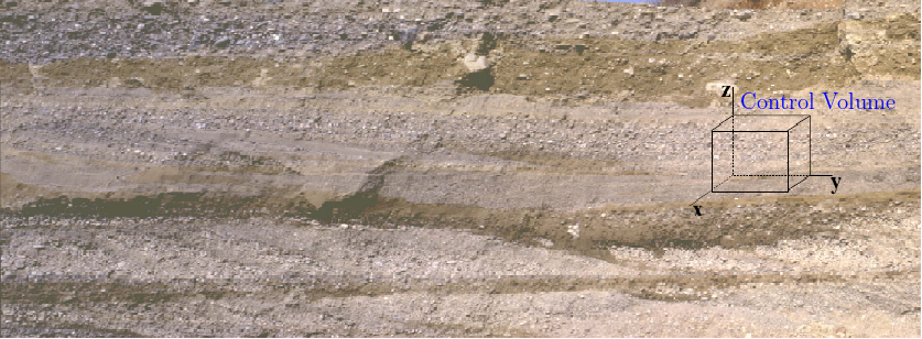
Fig. 6.1 A control volume#
6.2.2. Classification of Groundwater Flow Regimes#
Since we intend to formulate system equations for groundwater flow, it is important that we first classify the groundwater problems as per the flow regimes. In general such classification can contain:
Property |
Problem-Type |
|---|---|
Dimension-wise |
1D, 2D or 3D |
Time-function |
Stead-State or transient |
Space-dependent |
Homogeneous or heterogeneous |
Direction-dependent |
Isotropic or anisotropic |
Aquifer type |
Confined or unconfined |
Source function |
With or without source/sinks |
The combination presented in the table above amounts to 96 possible combinations and only very exceptional scenarios are possible. Each combination resulting from the table corresponds to a certain equation governing groundwater flow. Thus many similarities in formulation exist but only differences are with respect to details.
Attention
All the formulations of groundwater system equation are based on just two principles. They are:
The conservation of volume
Darcy’s law
The above two principles are sufficient for formulation of system equations for consolidated aquifers. The system equations for consolidated aquifers can be bit more complicated. This course only very limitedly deals with such aquifers.
6.2.3. Conservation of Volume#
Let us consider a control volume with inlet and outlet as shown in the figure below.
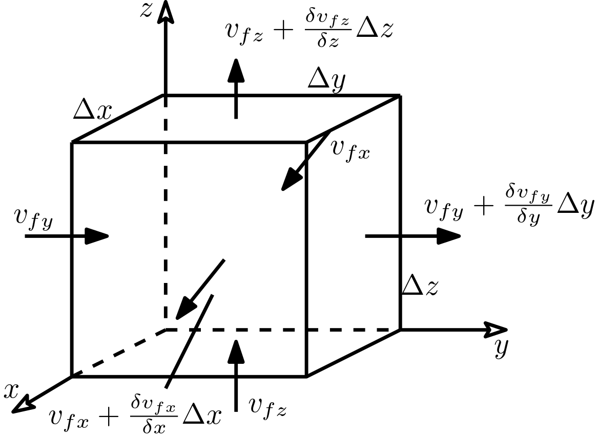
Fig. 6.2 Conservation of volume#
The volume budget in this control volume can be expressed as:
\begin{equation} \frac{\Delta V_w}{\Delta t} = Q_{in} - Q_{out} \end{equation}
The scenario that can be considered with the conservation of volume are:
3D
transient
isotropic
heterogeneous
confined
without sources/sinks
6.2.4. Darcy’s Law#
The generalized Darcy’s law is
where \(K\) when the principal axes not aligned to the domain coordinates is gives as (see Steady-State Groundwater flow in 3D)
It is to be noted that \(K\) is a scalar for isotropic aquifers and tensor (as above) for anisotropic aquifers. Further, in the Darcy’s law, the gradient vector [-] is oriented in the direction of the steepest increase in hydraulic head. The minus sign indicates that groundwater flow is directed from large to small head values.
6.2.5. Inflow and Outflow#
The importance of control volume can be now observed as we derive the system equations for groundwater flow. The control volume as stated earlier has a very small size compared to the region of investigation. This entails that the changes of Darcy velocity components across this volume can therefore considered to be linear, i.e., the flow components do not meander. With this assumption, the linear changes are obtained by multiplying first-order derivatives with corresponding distance (see figure below). Mathematically put we have
Fig. 6.3 Conservation of volume#
The sum of all discharge at the inlets:
The sum of all discharge at the outlets:
The different in discharge between inlet and outlet:
Now, as we discussed in Groundwater as a reservoir it is known that change in water volume in an specific volumetric space is
which was formulated as
That is, the value of the storage coefficient corresponds to the change in water volume within a unit control volume if hydraulic head is increased/decreased by one unit.
6.2.6. Budgeting#
Equations (1), (2) and (3) can be combined to obtain the expression for the water budget, i.e., rate of change of water volume, which is
letting \(\Delta t \to 0\), the above expression transforms to
Now, replacing Darcy’s velocity vector by components:
we get the a system equation for a groundwater flow as
Groundwater system equation for a 3D transient homogeneous and isotropic aquifers
6.2.7. Further Versions of the 3D Groundwater Flow Equation:#
The groundwater system equation derived above can be modified in several ways to align with the problem in question. Few modifications are presented below.
6.2.7.1. Inclusion of sources/sinks (\(q\))#
Source in groundwater system can be for example water transferred to groundwater from river or more often encountered case of water injection through wells. Similarly, sinks can be water abstraction or drainage of groundwater to the river (or any other surface water bodies). The sources/sinks can be represented by term \(q\) [1/T] in the groundwater system equation, which leads to
Note
There can be several sources and sinks term and they can be simply added to the equation. A care has to be taken on the dimension [1/T] of the sources and sinks
6.2.7.2. Inclusion of Anisotropy#
For simplicity, we assume that principal axes of anisotropy are in parallel with the coordinate axes. This makes the groundwater equation take the form:
Note
Every directional \(K\)’s have to be considered (see Steady-State Groundwater flow in 3D) if principal axes of anisotropy is not parallel with the considered coordinate axes.
6.2.8. Special Groundwater Problems and Their System Equations#
6.2.8.1. The Poisson equation#
The Poisson equation deals with groundwater problem with the following condition:
Steady-state
Homogeneous
Isotropic
Confined
Sources/sinks
The equation is given as
6.2.8.2. The Laplace equation#
The Laplace equation deals with groundwater problem with the following condition:
Steady-state
Homogeneous
Isotropic
Confined
Without sources/sinks
The equation is given as
6.3. Two-dimensional Groundwater Flow in Confined Aquifers#
For most unconsolidated aquifers it is observed that groundwater flow components perpendicular to layering are negligible (see figure below). Therefore, groundwater flow problems are frequently treated as two-dimensional, i.e., employing only two spaces coordinates.
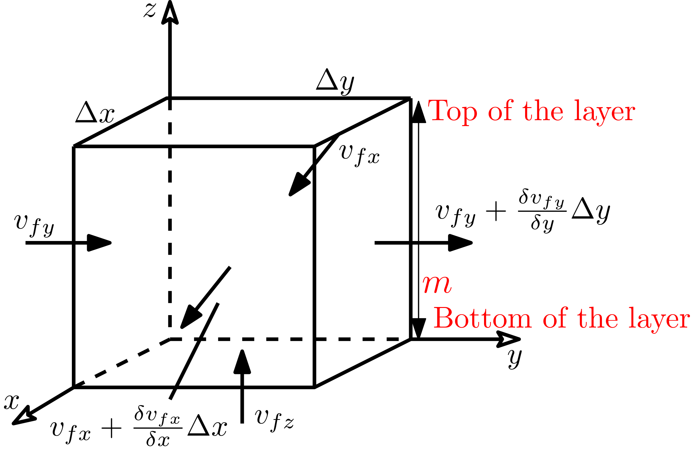
Fig. 6.4 2D- flow in confined aquifers#
The control volume in the confined aquifer is extended over the entire layer thickness of \(m\). If an aquifer consists of several distinct major layers, the two-dimensional approach is used for each layer separately and, in addition, water transfer between layers is handled by appropriate source/sink terms (not shown in figure).
The step from three to two dimensions requires to sum up hydraulic conductivity values over the entire layer thickness in order to correctly quantity two-dimensional groundwater flow. This is done by introducing transmissivities \(T_x\) and \(T_y\) [L2/T] as follows:
where \(K_x\) and \(K_y\) denote vertically averaged hydraulic conductivities [L/T] along the \(x-\) and \(y-\) coordinate, respectively. For a confined aquifer which is horizontally isotropic we simply have
6.3.1. Example problem#
Hydraulic gradient in 2D
Calculate the transmissivity for an isotropic confined aquifer.
print("\n\033[1mProvided are:\033[0m\n")

K = 5e-4 # m/s, hydraulic conductivity
m = 45 # m, aquifer thickness
print("hydraulic conductivity = {} m/s\naquifer thickness = {} m\n".format(K,m),)
Provided are:

hydraulic conductivity = 0.0005 m/s
aquifer thickness = 45 m
K = 5e-4 # m/s, hydraulic conductivity
m = 45 # m, aquifer thickness

#solution
T = K*m
print("\033[1mSolution:\033[0m\nThe resulting transmissivity is \033[1m{:02.4} m²/s\033[0m.".format(T))
Solution:
The resulting transmissivity is 0.0225 m²/s.
6.3.2. Example problem#
Hydraulic gradient in 2D
Calculate the transmissivity for an isotropic unconfined aquifer.
Provided are:

hydraulic conductivity = 0.0005 m/s
hydraulic head = 130 m
aquifer bottom elevation = 110 m
K = 5e-4 # m/s, hydraulich conducticity
h = 130 # m, hydraulic head
z_bot = 110 # m, aquifer bottom elevation

#solution
T = K*(h-z_bot)
print("\033[1mSolution:\033[0m\nThe resulting transmissivity is \033[1m{:02.4} m²/s\033[0m.".format(T))
Solution:
The resulting transmissivity is 0.01 m²/s.
6.3.3. 2D Groundwater Flow Equations for Confined Conditions#
As was mentioned in Groundwater as a reservoir, the storage coefficient \(S\) [-] is to be used instead of \(S_s\) [1/L] if vertical flow components are neglected. This results in the following 2D groundwater flow equations without sources/sinks:
The 2D groundwater flow equation with sources/sinks:
where \(N\) denotes the volumetric flux due to source/sinks per unit surface area [L/T].
6.4. Two-dimensional Groundwater Flow in Unconfined Aquifers#
For unconfined layers, the control volume extends from the aquifer bottom to the groundwater table (see figure below). This implies that the height of the control volume depends on the flow behaviour.
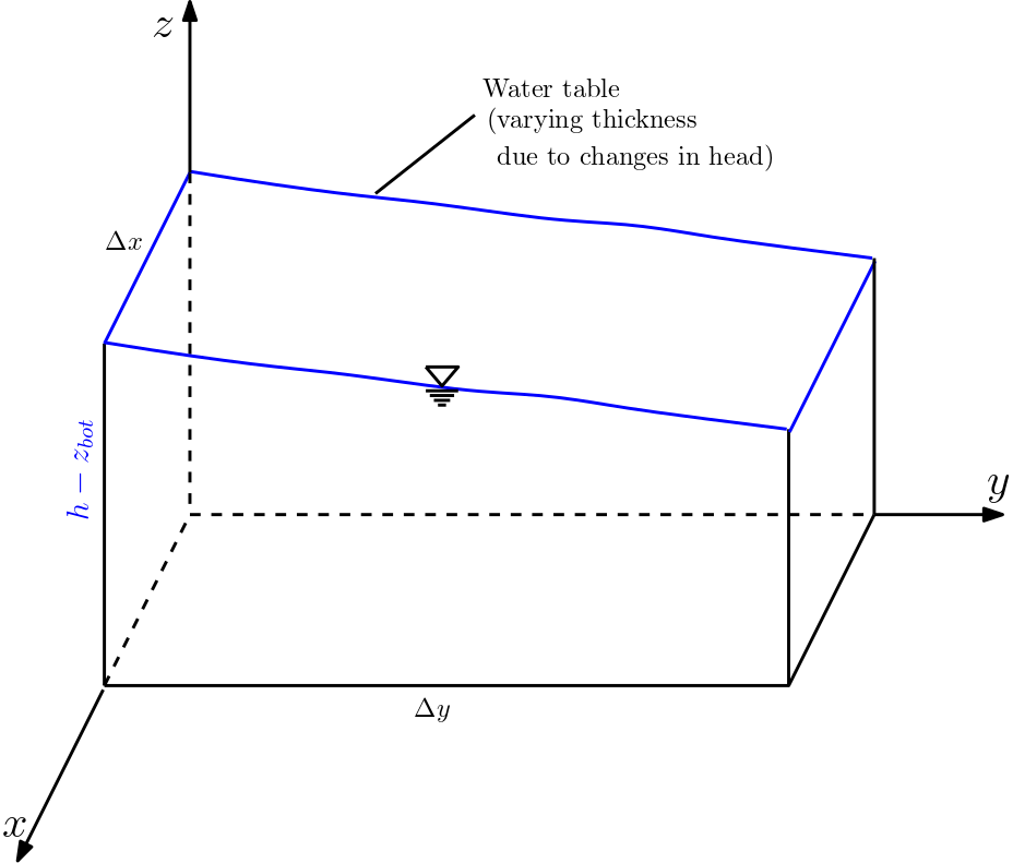
Fig. 6.5 2D- flow in unconfined aquifers#
Since the height of the control volume depends on the flow behaviour, the transmissivities are defined by using hydraulic head \(h\) to account for the saturated thickness:
where \(z_{bot}\) represents the elevation of the aquifer bottom [L]. Formally, the 2D groundwater flow equation for unconfined aquifers is the same as for the confined conditions, i.e.,
However, transmissivities are computed in a different way. The above equation is also termed Boussinesq equation.
6.4.1. Dupuit Assumptions#
The Boussinesq equation for 2D groundwater flow in unconfined aquifer is based on the following assumptions which are due to Dupuit (1863)1. The Dupuit’s work can be expressed in the figure below.
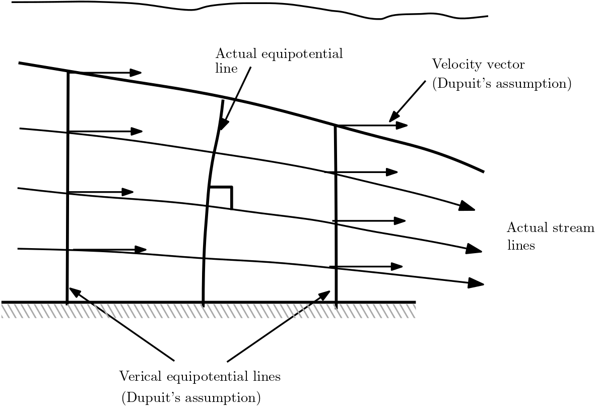
Fig. 6.6 Illustration of Dupuit’s assumptions#
The Dupuit’s assumptions are:
Groundwater flow is horizontal (no vertical flow components).
The flow velocity does not vary with depth.
Darcy’s law also holds at the water table.
6.5. Complete Formulation of Groundwater Flow Problems#
The complete formulation of groundwater flow requires following the specific steps. These are:
Step I : Specify the geometric properties of the region of interest (dimensionality, shape).
Step II : Specify values of aquifer parameters (hydraulic conductivity, storage coefficient) by considering spatial variability and anisotropy, if necessary.
Step III : Select the appropriate flow equation.
Step IV : Specify the initial condition. (IC):
A. head value at time. \(t=0\)
B. This step is not required for steady-state problems.
Step IV : Specify boundary conditions (BC):
A. BCs have to be given along the complete boundary (also at infinity if regions are assumed to be unbounded).
B. BCs may be time-dependent.
C. There are three major types of BCs .
6.5.1. Boundary Conditions#
The number of boundary conditions required corresponds to the highest space derivative for each coordinate in the flow equation. The three boundary conditions are:
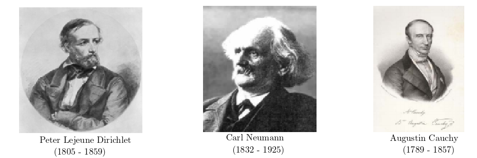
Boundary condition of the first kind or Dirichlet Boundary condition: - The head value is given.
Boundary condition of the second kind or Neumann Boundary condition: - The component of the head gradient, which is perpendicular to the boundary, is given.
Boundary condition of the third kind or Cauchy boundary condition or Robin boundary condition (for completeness only): - A relationship between the head value and the component of the head gradient, which is perpendicular to the boundary, is given.
6.5.2. Relationships Aquifer/Flow Property and Mathematical Formulation#
The following table summarizes the relationship between aquifer flow property and the corresponding mathematical formulation.
Aquifer/Flow property |
Mathematical Formulation |
|---|---|
Transient |
with time derivative |
Confined |
linear partial differential equation |
Anisotropic |
\(T_x \neq T_y\) or \(K_x \neq K_y\), resp. (tensor) |
Heterogeneous (inhomogeneous) |
coefficients depends on space coordinate(s) |
With sources/sinks |
inhomogeneous differential equation (contains a term without \(h\)) |
Fixed-head boundary condition |
boundary condition of the first kind (Dirichlet) |
Flux boundary condition (in particular: no flow) |
boundary condition of the second kind (Neumann) |
6.5.3. Implementing Groundwater Flow System Equation#
The figure below presents a groundwater problem with associated boundary conditions. The figure shows when a particular boundary condition is suitable. A zero flux or no flow boundary is streamline along boundaries 2-3 and 1-5. Likewise, the lake, whose water level can be constant is considered as prescribed head. From this example, it is evident that boundary conditions should be set based on geographical setting.
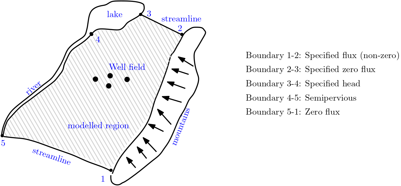
Fig. 6.7 Setting a groundwater problem (from Kinzelbach, 19862)#
The system equation including the boundary conditions makes a complete groundwater flow problem. The solution with inclusion of specific boundary conditions provides a unique or specific solution to the problem.
Numerical methods (discussed in lectures 11-13) are generally required to solve groundwater flow problems. In exceptional cases (e.g., single well, steady-state, isotropic and homogeneous), analytical solution are also possible (discussed in the next lecture).