Steady-State Groundwater flow in 3D
Contents
5. Steady-State Groundwater flow in 3D#
(The contents presented in this section were re-developed principally by Dr. P. K. Yadav. The original contents are from Prof. Rudolf Liedl)
5.1. Motivation#
This lecture shows how Darcy’s law can be used for variety of groundwater problems, e.g., in isotropic and anisotropic aquifers, multiple dimension problems - 2D and 3D. The lecture will also introduce the basic concepts on visualizing groundwater flow, e.g., using streamlines, flow-nets, and present their uses for example using isochrones and delineating protection zones.
5.2. Darcy’s Law in Isotropic Aquifers#
5.2.1. Summarizing Hydraulic Head#
The Darcy’s column experiment is associated with one-dimensional (1D) steady-state or time independent flow system. In addition, the experiments as we discussed in lecture 4, dealt with homogeneous (space dependency) and isotropic (direction dependency) porous media. The consequence of these is that the hydraulic head \(h\) in a Darcy column therefore depends on a single space coordinate, say \(x\) that is oriented along the column length. Therefore \(h = h(x)\) in this case.
Now considering the real/natural aquifer, which is inherently three dimensional (3D), the hydraulic head is then a function of three space coordinates, i.e., \(h = h(x,y,z)\). But the 3D natural problem can be simplified to 2D problems based on the fact that vertical flow components (e.g., the aquifer depth) is very much smaller than horizontal flow components (the aquifer width or its length), i.e., \(h = h(x,y)\) considering \(z\) as vertical components. The 2D approach, instead of 3D, has been found to appropriately quantify groundwater flow systems. The application of 2D or 1D for quantifying in groundwater flow system have be justified for each case. For example the layered aquifers, that was discussed in lecture 5, can be easily treated as a 2D system.
Note
The hydraulic head (\(h\)) in any case (1D, 2D or 3D), is the sum of hydrostatic pressure head (\(\psi\)) and the elevation head (\(z\)) and has a dimension of length [L], i.e.,
5.3. Isolines and Isosurfaces#
We make a slight detour from the Darcy’s law and quantifying groundwater flow system to visualizing the groundwater flow. As can be expected, visualizing groundwater is a challenging task. This is largely because sub-surface, compared to surface, cannot be mapped with very high resolution. However, it is possible to connect aquifer properties such as \(h\) hydraulic head to visualize groundwater flow system. Particularly used to visualize groundwater are:
Isolines: The curves (in 2D space) where a physical quantity (e.g., \(h\)) assumes a certain value. Isolines are thus suitable for visualizing 2D problems.
Isosurface: The surfaces (in 3D space) where a physical quantity assumes a certain value. Isosurface addresses the 3D groundwater problems.
The representation of isolines yields a map. Isolines are therefore frequently superimposed on an already existing geographical map, e.g., the topographical map (see Fig. 5.1). The simultaneous representation of several isolines/isosurfaces can be confusing. Thus intervals between values represented by these representations are constant.
Isosurfaces are in general confusing to interpret due to presence of the third dimensions. As such often 2D cross-section through isosurfaces are depicted.
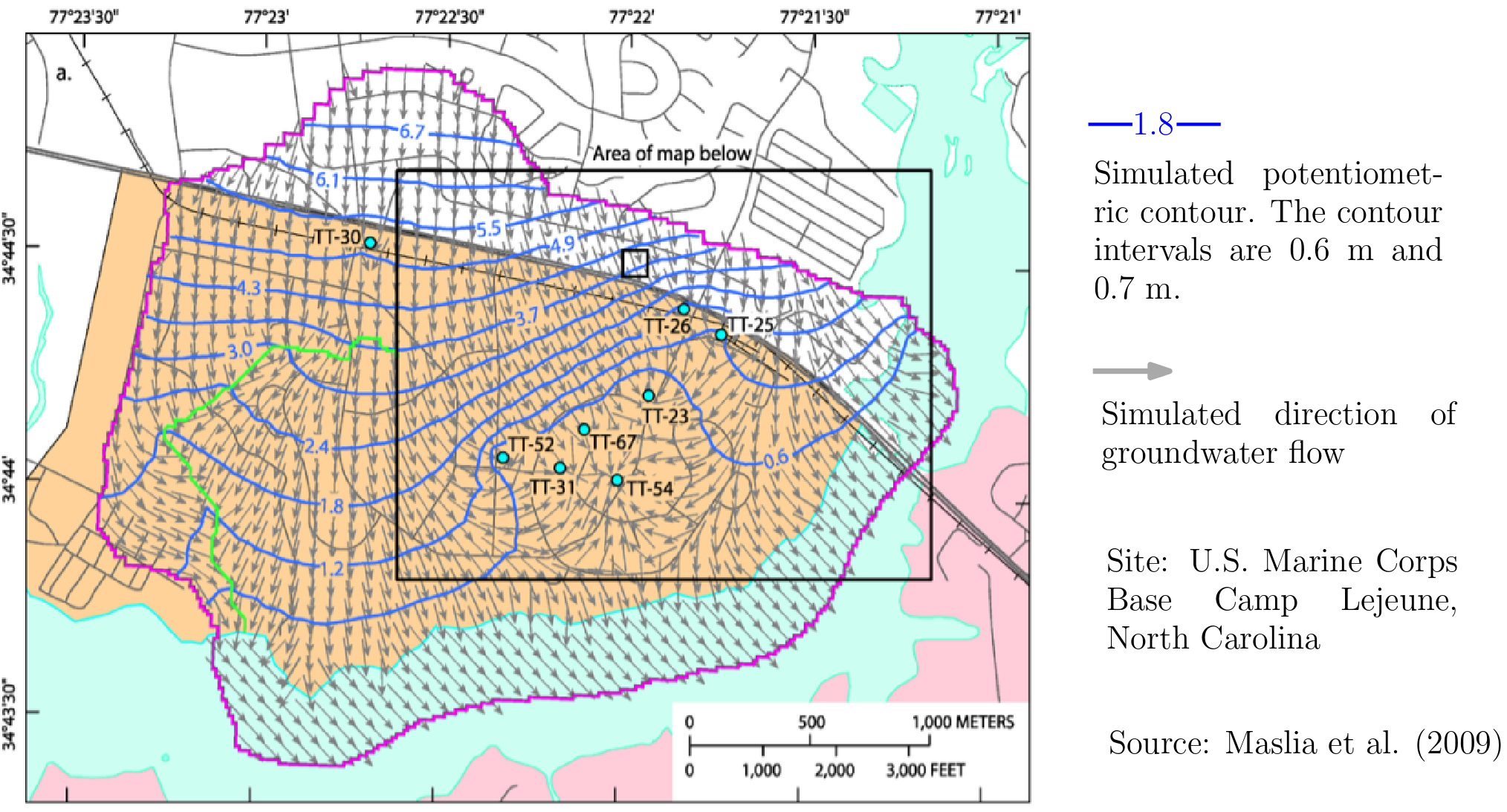
Fig. 5.1 Head Isolines#
5.4. Hydrologic Triangle#
The hydrologic triangle is a method that is used to approximate head isolines when head values are available at some distinct locations. As the name suggests, at least three head data are required to be known for approximating isolines. The process used in approximating is as follows:
First the known head data points are connected with straight lines (dashed lines in the figure Fig. 5.2).
Linear interpolation is then performed with pre-defined head intervals (\( \Delta h = 1 m \) in the figure).
Finally, points with identical head values are connected to obtain the isolines (solid lines in the figure).
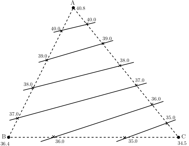
Fig. 5.2 Hydrologic Triangle#
5.4.1. Applying the Hydrologic Triangle#
In practical cases more than the just three observation points are available. This implies a triangulation of the investigation area as shown in the figure (Fig. 5.3). Linear interpolation of heads is again performed along the dashed lines. Points with identical head values are connected to obtain the isolines. The connection lines do not have to be strictly a straight line as was the case in Fig. 5.2. In addition to straight line segments, the connected line can be smooth curves as shown in the Fig. 5.3.
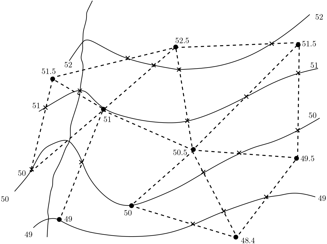
Fig. 5.3 Applying the Hydrologic Triangle#
5.4.2. Flow Direction#
Based on Darcy’s law it is known that the flow is directed from the higher head towards the lower head. Though Darcy’s law is based on 1D, the same concept can be extended to the 2D and 3D flow. Thus in the figure, (Fig. 5.4), the flow direction can be assumed to be directed from the top towards the base of the triangle (red arrow in the figure). But this remains assumptions so far.
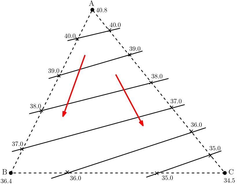
Fig. 5.4 Flow Direction in Hydrologic Triangle#
Attention
What is the correct extension of Darcy’s law- in 2D and 3D systems?
5.5. Hydraulic Gradient in 2D and 3D systems#
The hydraulic gradient appears as a major constituent of Darcy’s law for 1D flow. In the 1D case the hydraulic gradient is given as the ratio of difference of heads at two points in the space and the distance between those points. This distance measures also the flow length. Since head is direction oriented, the hydraulic gradient in the 2D or the 3D flow must be a vector quantity. This combines both magnitude and direction that fits the definition of hydraulic gradient. Therefore hydraulic gradient in 2D or 3D is achieved by employing partial derivatives of hydraulic head with respect to Cartesian coordinates. Mathematically, this can be represented as:
\(\text{grad}h\) in the equation above is a vector pointing in the direction of the steepest increase of \(h\). In groundwater/hydrogeology study, in contrast to the mathematical definition, \(\text{grad}h\) refer to the direction of steepest decrease of hydraulic head. This can be observed in Fig. 5.1
5.5.1. Darcy’s Law (Isotropic Aquifer)#
The concept used for hydraulic gradient for 2D/3D discussed above can be extended to specific discharge or Darcy velocity \(v_f\). Similar to hydraulic gradient, \(v_f\) is a vector with two or three components for 2D and 3D systems, respectively. Thus the 3D Darcy velocity vector is
Therefore in higher dimension systems, the Darcy law can be stated as
Based on this definition, the hydraulic conductivity (\(K\)) is
Heterogeneous aquifer: \(K = K(x,y,z\), and
Homogeneous aquifer: \(K = \text{constant}\)
For isotropic aquifers the Darcy velocity is oriented opposite to the hydraulic gradient vector (due to minus sign in Darcy’s law). This is explained further below.
5.5.2. Example problem#
Hydraulic gradient in 2D
Obtain the hydraulic gradients of the following 2D system shown in the figure below
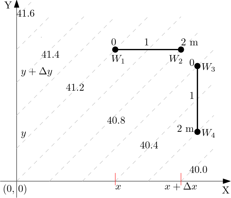
Fig. 5.5 Example 1#
Solution
Known for the 2D system is:
In which for fixed \(y\),
and for fixed \(x\),
Then from the given figure:
# solution

import numpy as np

h_xdelx = 40.8 # m, head at W2
h_x = 41.2 # m, head at W1
Lx = 2 # m, length between W1 and W2

h_xdely = 40.6 # m, head at W2
h_y = 40.2 # m, head at W1
Ly = 2 # m, length between W1 and W2

# calculate
Delh_x = (h_xdelx - h_x)/Lx # (-), hydraulic head along x-axis
Delh_y = (h_xdely - h_y)/Ly # (-), hydraulic head along y-axis

#print
print("Hydraulic gradient along x-axis is {0:0.3f}\n".format(Delh_x))
print("Hydraulic gradient along y-axis is {0:0.3f}\n".format(Delh_y))
Hydraulic gradient along x-axis is -0.200

Hydraulic gradient along y-axis is 0.200
Attention
In the above example the orientation of co-ordinate axis is important. The change in orientation of axis, e.g., \(y\)-axis pointing downward will make also hydraulic gradient along \(y\) negative.
5.6. Streamlines and Flow Nets#
5.6.1. Basics#
Streamlines or flowlines are curves which are in each point tangential to the flow direction. There is no flow component perpendicular to the streamlines. As a consequence, streamlines are perpendicular to head iso-surface of head isolines if the aquifer is isotropic
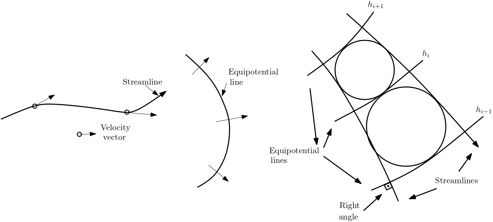
Fig. 5.6 Streamlines and equipotential lines#
Flow nets consist of a set of isolines (or isosurfaces) and a set of streamlines. Flow nets are ususally employed for 2D flow scenarios only. The flow behaviour is illustrated by covering the investigation area with a mesh of isolines and streamlines.
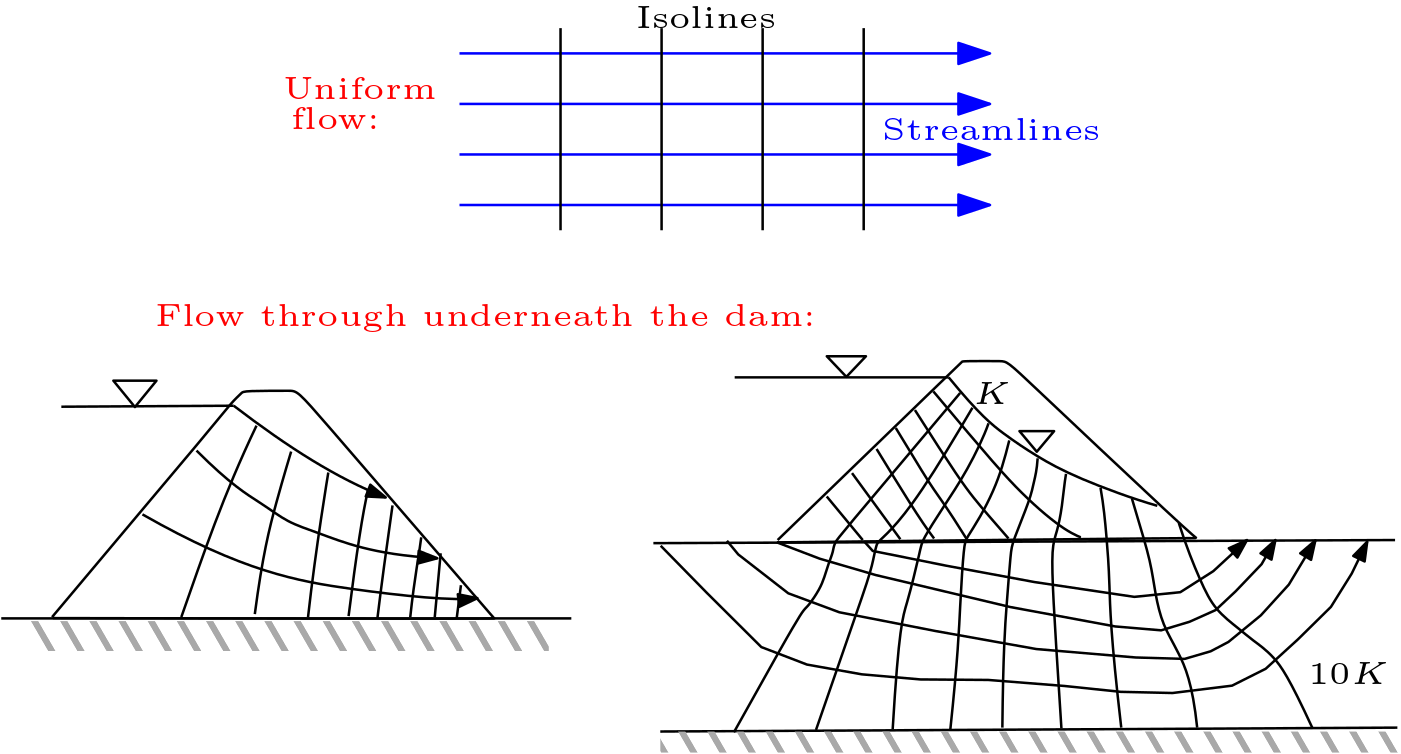
Fig. 5.7 Flow nets#
5.6.2. Radial Flow Near a Well#
In this example steady-state water abstraction from a pumping well, e.g., for drinking water supply, is considered. The hydraulic conductivity is assumed to be spatially constant, i.e., the aquifer is homogeneous. Now assuming that there are no other hydraulic impacts in the system, the pumping of water from the groundwater will lead to a radially symmetric drawdown of hydraulic heads (this will be further discussed in future lecture 8). In this case the streamlines radially approaches the pumping well, and the head isolines are circles with the well in the centre.
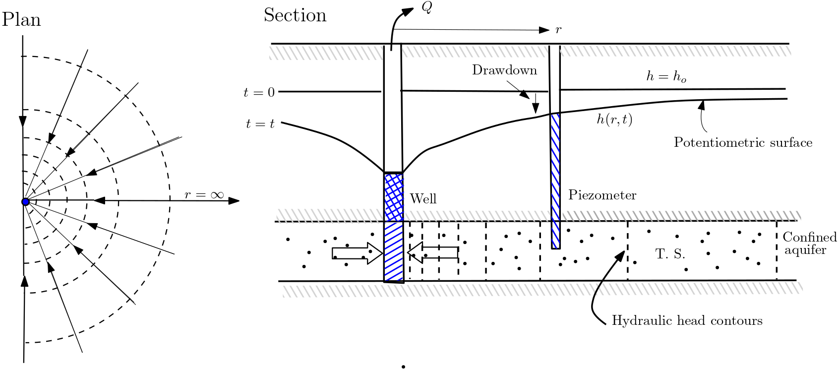
Fig. 5.8 Radial flow near a well#
5.6.3. Superposition of Uniform and Radial Flow#
The dividing streamline (solid black line) represents the boundary of the well capture zone. The flow velocities of the uniform flow and the radial flow exactly compensate each other at the stagnation point. The resulting flow velocity equal zero.
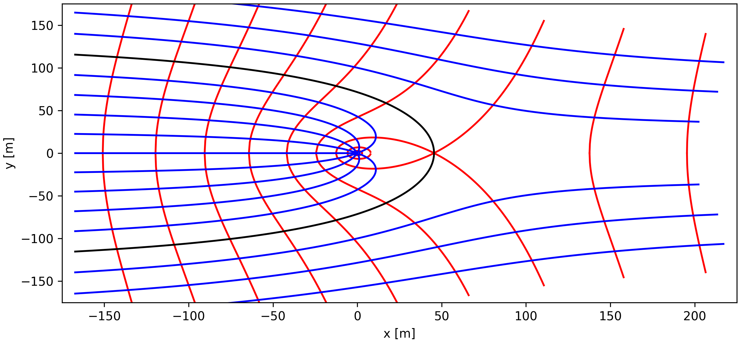
Fig. 5.9 Superposition of Radial flow near a well#
5.6.4. Some Rules for Drawing Flow Nets#
Drawing a flow net for a certain domain requires information about domain boundaries.
Impermeable boundaries represents a streamline.
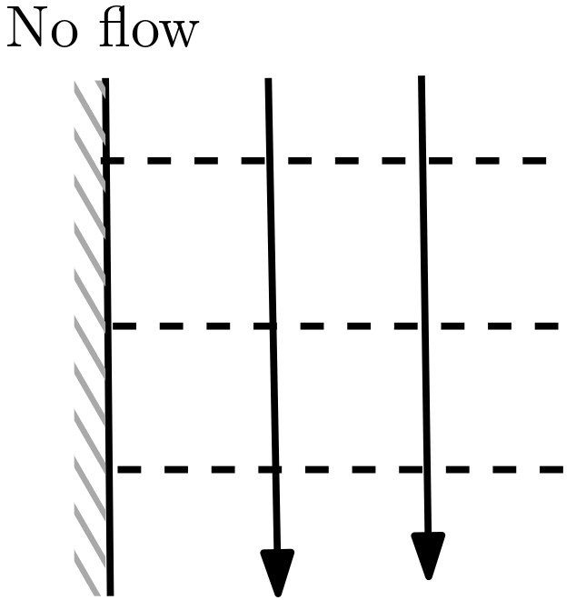
Fig. 5.10 No flow boundary#
Constant head boundaries with given head values represents isolines.
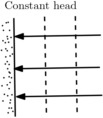
Fig. 5.11 Constant head boundary#
Water table with and without evapotranspiration and recharge: Isolines and streamlines are drawn only for the saturated zone, i.e., they do not cross the water table.
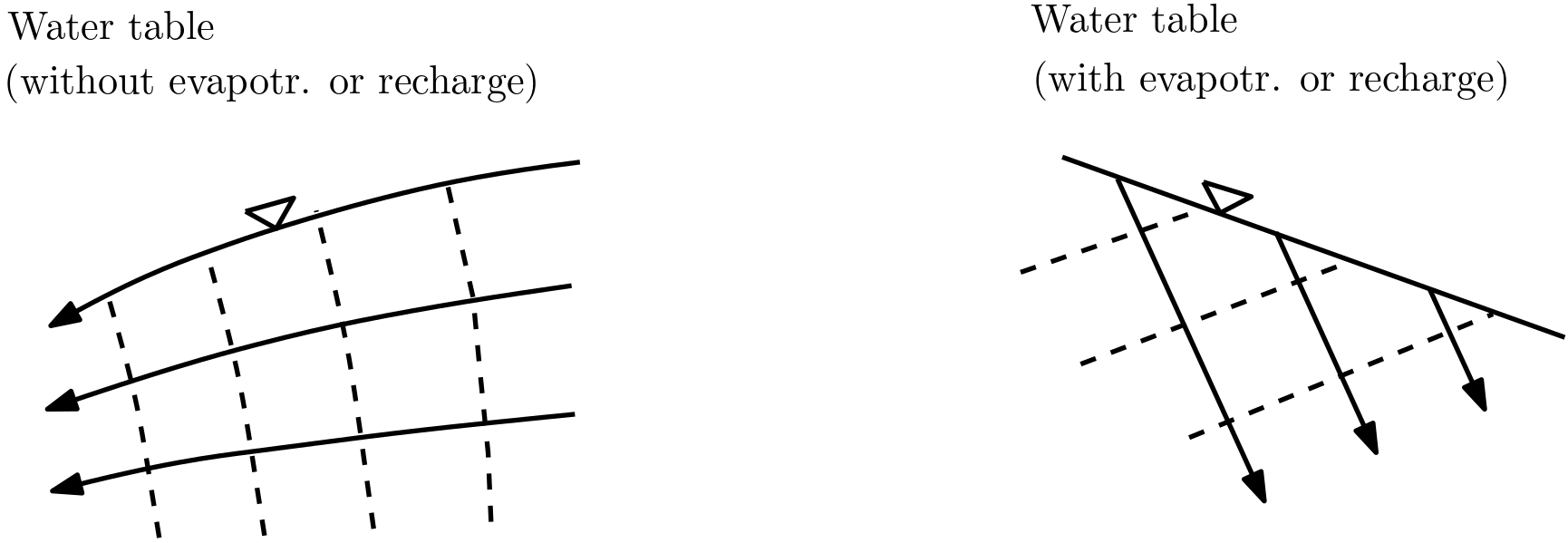
Fig. 5.12 Water table as boundary#
Isolines do not intersect each other. Streamlines do not intersect each other.
Streamlines are never closed (circular). They start at an inflow boundary and end at an outflow boundary.
Adjacent isolines and streamlines should form curvilinear squares.
5.6.5. Example problem#
Flow parallel to layering
Considering \(K = 6\) cm/s and \(w = 50 \)cm, the width normal to plane, find the total discharge from the flow net provided in figure below:
(source: https://gw-project.org/)
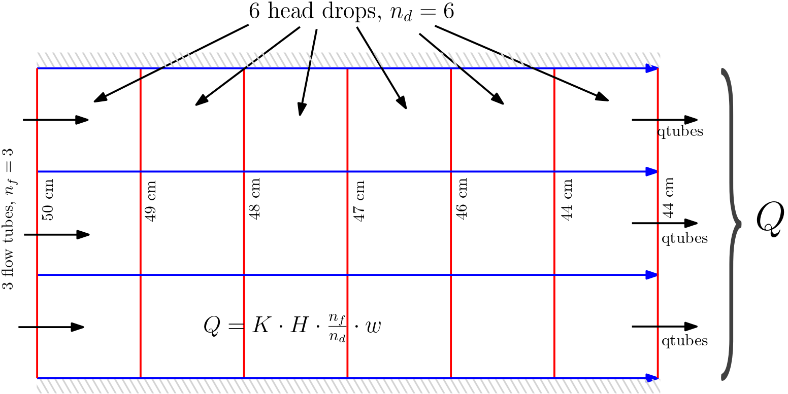
Fig. 5.13 Example problem 2
#
### solution

n_f = 3 # numer of flow tubes
n_d = 6 # number of head drops in the flow net
w = 50 # cm, width lateral to the plane
K = 0.4 # cm/s, conductivity
h_in = 50 # cm, head inlet
h_out = 44 # cm, head outlet

#interim calculation
H = h_in-h_out

Q_t = K*H*n_f/n_d*w # cm^3/s, the total discharge

print("The total discharge out of domain is {0:0.0f}".format(Q_t), "cm\u00b3/s")
The total discharge out of domain is 60 cm³/s
5.7. Isochrones and Protection Zones.#
5.7.1. Ischrones#
The isochrones are curves of identical travel times. This is analogous to head isolines, in which the curves provides point of identical head. Similar to isolines, isochrones and streamlines do not necessarily intersect each other at an angle of 90\(^\circ\), i.e., curvilinear intersection between these curves are also possible.Isochrones are mostly used for delineating water protection zones. These zones are mostly part of the local water-use regulations.
import numpy as np
from ipywidgets import *
import matplotlib.pyplot as plt

import warnings
warnings.filterwarnings('ignore')

#definition of the function
def uniform_flow(K, ne, m, v, Q, t1, t2, t3):

    #intermediate results
    K_1 = K*86400                       #hydraulic conductivity [m/d]
    capture_width = Q/m/v               #capture width [m]
    L_ref = Q/(2*np.pi*np.exp(1)*m*v)   #[m]
    h_ref = v/K_1*L_ref                 #[m]
    t_ref = 0.5*ne*Q/np.pi/m/v**2       #[d]
    stagnation_x = np.exp(1)*L_ref      #stagnation point (x) [m]
    stagnation_y = 0                    #stagnation point (y) [m]

    #isolines; Syntax: isolines_[X or Y]_plot_[h_ref]_[optional: 1 or 2]
    isolines_x_plot_n5_1=[]
    isolines_y_plot_n5_1=[]
    isolines_x_plot_n5_2 = []
    isolines_y_plot_n5_2 = []
    isolines_x_plot_n2_5_1 = []
    isolines_y_plot_n2_5_1 = []
    isolines_x_plot_n2_5_2 = []
    isolines_y_plot_n2_5_2 = []
    isolines_x_plot_0_1 = []
    isolines_y_plot_0_1 = []
    isolines_x_plot_0_2 = []
    isolines_y_plot_0_2 = []
    isolines_x_plot_2_5 = []
    isolines_y_plot_2_5 = []
    isolines_x_plot_5 = []
    isolines_y_plot_5 = []
    isolines_x_plot_7_5 = []
    isolines_y_plot_7_5 = []
    isolines_x_plot_10 = []
    isolines_y_plot_10 = []
    isolines_x_plot_12_5 = []
    isolines_y_plot_12_5 = []
    isolines_x_plot_15 = []
    isolines_y_plot_15 = []


    for x in range(0, 100):
        isolines_x_n5_1=L_ref*((x*0.169103048517306+(100-x)*-0.150360933444141)/100)
        isolines_x_n5_2=L_ref*((x*12.35+(100-x)*11.6815653622516)/100)
        isolines_x_n2_5_1=L_ref*((x*0.474722923528955+(100-x)*-0.350418198256065)/100)
        isolines_x_n2_5_2=L_ref*((x*9.45+(100-x)*8.22933315122817)/100)
        isolines_x_0_1=L_ref*((x*np.exp(1)+(100-x)*-0.75695357132717)/100)
        isolines_x_0_2=L_ref*((x*6.65+(100-x)*np.exp(1))/100)
        isolines_x_2_5=L_ref*((x*4+(100-x)*-1.46395392968976)/100)
        isolines_x_5=L_ref*((x*1.5+(100-x)*-2.50444142220744)/100)
        isolines_x_7_5=L_ref*((x*-0.875+(100-x)*-3.84154019983304)/100)
        isolines_x_10=L_ref*((x*-3.15+(100-x)*-5.4105773228373)/100)
        isolines_x_12_5=L_ref*((x*-5.4+(100-x)*-7.15205676143326)/100)
        isolines_x_15=L_ref*((x*-7.65+(100-x)*-9.02099613666581)/100)

        if x == 0:
            isolines_y_n5_1 = 0
            isolines_y_n5_2 = 0
            isolines_y_n2_5_1 = 0
            isolines_y_n2_5_2 = 0
            isolines_y_0_1 = 0
            isolines_y_0_2 = 0
            isolines_y_2_5 = 0
            isolines_y_5 = 0
            isolines_y_7_5 = 0
            isolines_y_10 = 0
            isolines_y_12_5 = 0
            isolines_y_15 = 0

        else:
            isolines_y_n5_1 = np.sqrt((L_ref*np.exp(-5/np.exp(1)+isolines_x_n5_1/L_ref/np.exp(1)))**2-isolines_x_n5_1**2)
            isolines_y_n5_2 = np.sqrt((L_ref*np.exp(-5/np.exp(1)+isolines_x_n5_2/L_ref/np.exp(1)))**2-isolines_x_n5_2**2)
            isolines_y_n2_5_1 = np.sqrt((L_ref*np.exp(-2.5/np.exp(1)+isolines_x_n2_5_1/L_ref/np.exp(1)))**2-isolines_x_n2_5_1**2)
            isolines_y_n2_5_2 = np.sqrt((L_ref*np.exp(-2.5/np.exp(1)+isolines_x_n2_5_2/L_ref/np.exp(1)))**2-isolines_x_n2_5_2**2)
            isolines_y_0_1 = np.sqrt((L_ref*np.exp(0/np.exp(1)+isolines_x_0_1/L_ref/np.exp(1)))**2-isolines_x_0_1**2)
            isolines_y_0_2 = np.sqrt((L_ref*np.exp(0/np.exp(1)+isolines_x_0_2/L_ref/np.exp(1)))**2-isolines_x_0_2**2)
            isolines_y_2_5 = np.sqrt((L_ref*np.exp(2.5/np.exp(1)+isolines_x_2_5/L_ref/np.exp(1)))**2-isolines_x_2_5**2)
            isolines_y_5 = np.sqrt((L_ref*np.exp(5/np.exp(1)+isolines_x_5/L_ref/np.exp(1)))**2-isolines_x_5**2)
            isolines_y_7_5 = np.sqrt((L_ref*np.exp(7.5/np.exp(1)+isolines_x_7_5/L_ref/np.exp(1)))**2-isolines_x_7_5**2)
            isolines_y_10 = np.sqrt((L_ref*np.exp(10/np.exp(1)+isolines_x_10/L_ref/np.exp(1)))**2-isolines_x_10**2)
            isolines_y_12_5 = np.sqrt((L_ref*np.exp(12.5/np.exp(1)+isolines_x_12_5/L_ref/np.exp(1)))**2-isolines_x_12_5**2)
            isolines_y_15 = np.sqrt((L_ref*np.exp(15/np.exp(1)+isolines_x_15/L_ref/np.exp(1)))**2-isolines_x_15**2)

        isolines_x_plot_n5_1.append(isolines_x_n5_1)
        isolines_y_plot_n5_1.append(isolines_y_n5_1)
        isolines_x_plot_n5_2.append(isolines_x_n5_2)
        isolines_y_plot_n5_2.append(isolines_y_n5_2)
        isolines_x_plot_n2_5_1.append(isolines_x_n2_5_1)
        isolines_y_plot_n2_5_1.append(isolines_y_n2_5_1)
        isolines_x_plot_n2_5_2.append(isolines_x_n2_5_2)
        isolines_y_plot_n2_5_2.append(isolines_y_n2_5_2)
        isolines_x_plot_0_1.append(isolines_x_0_1)
        isolines_y_plot_0_1.append(isolines_y_0_1)
        isolines_x_plot_0_2.append(isolines_x_0_2)
        isolines_y_plot_0_2.append(isolines_y_0_2)
        isolines_x_plot_2_5.append(isolines_x_2_5)
        isolines_y_plot_2_5.append(isolines_y_2_5)
        isolines_x_plot_5.append(isolines_x_5)
        isolines_y_plot_5.append(isolines_y_5)
        isolines_x_plot_7_5.append(isolines_x_7_5)
        isolines_y_plot_7_5.append(isolines_y_7_5)
        isolines_x_plot_10.append(isolines_x_10)
        isolines_y_plot_10.append(isolines_y_10)
        isolines_x_plot_12_5.append(isolines_x_12_5)
        isolines_y_plot_12_5.append(isolines_y_12_5)
        isolines_x_plot_15.append(isolines_x_15)
        isolines_y_plot_15.append(isolines_y_15)

    #streamlines; synthax: streamlines_[X or Y]_plot_[psi]
    streamlines_x_plot_0 = [0, (L_ref*-10)]
    streamlines_y_plot_0 = [0, 0]
    streamlines_x_plot_0_2 = []
    streamlines_y_plot_0_2 = []
    streamlines_x_plot_0_4 = []
    streamlines_y_plot_0_4 = []
    streamlines_x_plot_0_6 = []
    streamlines_y_plot_0_6 = []
    streamlines_x_plot_0_8 = []
    streamlines_y_plot_0_8 = []
    streamlines_x_plot_1 = []
    streamlines_y_plot_1 = []
    streamlines_x_plot_1_2 = []
    streamlines_y_plot_1_2 = []
    streamlines_x_plot_1_4 = []
    streamlines_y_plot_1_4 = []
    streamlines_x_plot_1_6 = []
    streamlines_y_plot_1_6 = []

    for x in range(0,100):
        streamlines_y_0_2 = L_ref*((x*0+(100-x)*1.34462005667342)/100)
        streamlines_y_0_4 = L_ref*((x*0+(100-x)*2.6992421745751)/100)
        streamlines_y_0_6 = L_ref*((x*0+(100-x)*4.07255559164565)/100)
        streamlines_y_0_8 = L_ref*((x*0+(100-x)*5.47097889806004)/100)
        streamlines_y_1 = L_ref*((x*0+(100-x)*6.89826117541355)/100)
        streamlines_y_1_2 = L_ref*((x*2.13413758353342+(100-x)*8.35561532789609)/100)
        streamlines_y_1_4 = L_ref*((x*4.24381382643103+(100-x)*9.8422946888304)/100)
        streamlines_y_1_6 = L_ref*((x*6.31283612436048+(100-x)*11.3562442221618)/100)

        streamlines_x_0_2 = streamlines_y_0_2/np.tan(streamlines_y_0_2/L_ref/np.exp(1)-np.pi*0.2)
        streamlines_x_0_4 = streamlines_y_0_4/np.tan(streamlines_y_0_4/L_ref/np.exp(1)-np.pi*0.4)
        streamlines_x_0_6 = streamlines_y_0_6/np.tan(streamlines_y_0_6/L_ref/np.exp(1)-np.pi*0.6)
        streamlines_x_0_8 = streamlines_y_0_8/np.tan(streamlines_y_0_8/L_ref/np.exp(1)-np.pi*0.8)
        streamlines_x_1 = streamlines_y_1/np.tan(streamlines_y_1/L_ref/np.exp(1)-np.pi*1)
        streamlines_x_1_2 = streamlines_y_1_2/np.tan(streamlines_y_1_2/L_ref/np.exp(1)-np.pi*1.2)
        streamlines_x_1_4 = streamlines_y_1_4/np.tan(streamlines_y_1_4/L_ref/np.exp(1)-np.pi*1.4)
        streamlines_x_1_6 = streamlines_y_1_6/np.tan(streamlines_y_1_6/L_ref/np.exp(1)-np.pi*1.6)

        streamlines_x_plot_0_2.append(streamlines_x_0_2)
        streamlines_y_plot_0_2.append(streamlines_y_0_2)
        streamlines_x_plot_0_4.append(streamlines_x_0_4)
        streamlines_y_plot_0_4.append(streamlines_y_0_4)
        streamlines_x_plot_0_6.append(streamlines_x_0_6)
        streamlines_y_plot_0_6.append(streamlines_y_0_6)
        streamlines_x_plot_0_8.append(streamlines_x_0_8)
        streamlines_y_plot_0_8.append(streamlines_y_0_8)
        streamlines_x_plot_1.append(streamlines_x_1)
        streamlines_y_plot_1.append(streamlines_y_1)
        streamlines_x_plot_1_2.append(streamlines_x_1_2)
        streamlines_y_plot_1_2.append(streamlines_y_1_2)
        streamlines_x_plot_1_4.append(streamlines_x_1_4)
        streamlines_y_plot_1_4.append(streamlines_y_1_4)
        streamlines_x_plot_1_6.append(streamlines_x_1_6)
        streamlines_y_plot_1_6.append(streamlines_y_1_6)

    #isochrones
    isochrones_x_plot_t1 = []
    isochrones_y_plot_t1 = []
    isochrones_x_plot_t2 = []
    isochrones_y_plot_t2 = []
    isochrones_x_plot_t3 = []
    isochrones_y_plot_t3 = []

    #iterate 5 times with start value t_xmin1/ t_xmax1

    t1_xmin1=-np.exp(1)*np.sqrt(np.exp(2*(t1/t_ref))-1)
    t1_xmin6= t1_xmin1+(np.exp(1)-t1_xmin1)*(1+np.exp(1)/t1_xmin1*(np.log(1-t1_xmin1/np.exp(1))+(t1/t_ref)))
    t1_xmax1= np.exp(1)*np.sqrt(1-np.exp(-2*(t1/t_ref)))
    t1_xmax6= t1_xmax1+(np.exp(1)-t1_xmax1)*(1+np.exp(1)/t1_xmax1*(np.log(1-t1_xmax1/np.exp(1))+(t1/t_ref)))
    t2_xmin1=-np.exp(1)*np.sqrt(np.exp(2*(t2/t_ref))-1)
    t2_xmin6= t2_xmin1+(np.exp(1)-t2_xmin1)*(1+np.exp(1)/t2_xmin1*(np.log(1-t2_xmin1/np.exp(1))+(t2/t_ref)))
    t2_xmax1=np.exp(1)*np.sqrt(1-np.exp(-2*(t2/t_ref)))
    t2_xmax6= t2_xmax1+(np.exp(1)-t2_xmax1)*(1+np.exp(1)/t2_xmax1*(np.log(1-t2_xmax1/np.exp(1))+(t2/t_ref)))
    t3_xmin1=-np.exp(1)*np.sqrt(np.exp(2*(t3/t_ref))-1)
    t3_xmin6= t3_xmin1+(np.exp(1)-t3_xmin1)*(1+np.exp(1)/t3_xmin1*(np.log(1-t3_xmin1/np.exp(1))+(t3/t_ref)))
    t3_xmax1=np.exp(1)*np.sqrt(1-np.exp(-2*(t3/t_ref)))
    t3_xmax6= t3_xmax1+(np.exp(1)-t3_xmax1)*(1+np.exp(1)/t3_xmax1*(np.log(1-t3_xmax1/np.exp(1))+(t3/t_ref)))
    for i in range(4):
        t1_xmin6= t1_xmin6+(np.exp(1)-t1_xmin6)*(1+np.exp(1)/t1_xmin6*(np.log(1-t1_xmin6/np.exp(1))+(t1/t_ref)))
        t1_xmax6= t1_xmax6+(np.exp(1)-t1_xmax6)*(1+np.exp(1)/t1_xmax6*(np.log(1-t1_xmax6/np.exp(1))+(t1/t_ref)))
        t2_xmin6= t2_xmin6+(np.exp(1)-t2_xmin6)*(1+np.exp(1)/t2_xmin6*(np.log(1-t2_xmin6/np.exp(1))+(t2/t_ref)))
        t2_xmax6= t2_xmax6+(np.exp(1)-t2_xmax6)*(1+np.exp(1)/t2_xmax6*(np.log(1-t2_xmax6/np.exp(1))+(t2/t_ref)))
        t3_xmin6= t3_xmin6+(np.exp(1)-t3_xmin6)*(1+np.exp(1)/t3_xmin6*(np.log(1-t3_xmin6/np.exp(1))+(t3/t_ref)))
        t3_xmax6= t3_xmax6+(np.exp(1)-t3_xmax6)*(1+np.exp(1)/t3_xmax6*(np.log(1-t3_xmax6/np.exp(1))+(t3/t_ref)))

    for x in range (0,100):

        isochrones_x_t1 = 0.5*L_ref*(t1_xmin6+t1_xmax6+(t1_xmax6-t1_xmin6)*np.cos(np.pi*(100-x)/100))
        isochrones_x_t2 = 0.5*L_ref*(t2_xmin6+t2_xmax6+(t2_xmax6-t2_xmin6)*np.cos(np.pi*(100-x)/100))
        isochrones_x_t3 = 0.5*L_ref*(t3_xmin6+t3_xmax6+(t3_xmax6-t3_xmin6)*np.cos(np.pi*(100-x)/100))

        if x == 0:
            isochrones_y_t1 = 0
            isochrones_y_t2 = 0
            isochrones_y_t3 = 0
        else:

            isochrones_y1_t1 = L_ref*np.exp(1)*np.arccos((0.5*isochrones_x_t1/np.exp(1)/L_ref+np.exp(-(t1/t_ref)-isochrones_x_t1/np.exp(1)/L_ref))/(1-0.5*isochrones_x_t1/np.exp(1)/L_ref))
            isochrones_y_t1 = L_ref*np.exp(1)*np.arccos((isochrones_x_t1/L_ref*(np.sin(isochrones_y1_t1/np.exp(1)/L_ref)/(isochrones_y1_t1/L_ref)-0.5*np.cos(isochrones_y1_t1/np.exp(1)/L_ref)/np.exp(1))+np.exp(-(t1/t_ref)-isochrones_x_t1/np.exp(1)/L_ref))/(1-0.5*isochrones_x_t1/np.exp(1)/L_ref))

            isochrones_y1_t2 = L_ref*np.exp(1)*np.arccos((0.5*isochrones_x_t2/np.exp(1)/L_ref+np.exp(-(t2/t_ref)-isochrones_x_t2/np.exp(1)/L_ref))/(1-0.5*isochrones_x_t2/np.exp(1)/L_ref))
            isochrones_y_t2 = L_ref*np.exp(1)*np.arccos((isochrones_x_t2/L_ref*(np.sin(isochrones_y1_t2/np.exp(1)/L_ref)/(isochrones_y1_t2/L_ref)-0.5*np.cos(isochrones_y1_t2/np.exp(1)/L_ref)/np.exp(1))+np.exp(-(t2/t_ref)-isochrones_x_t2/np.exp(1)/L_ref))/(1-0.5*isochrones_x_t2/np.exp(1)/L_ref))

            isochrones_y1_t3 = L_ref*np.exp(1)*np.arccos((0.5*isochrones_x_t3/np.exp(1)/L_ref+np.exp(-(t3/t_ref)-isochrones_x_t3/np.exp(1)/L_ref))/(1-0.5*isochrones_x_t3/np.exp(1)/L_ref))
            isochrones_y_t3 = L_ref*np.exp(1)*np.arccos((isochrones_x_t3/L_ref*(np.sin(isochrones_y1_t3/np.exp(1)/L_ref)/(isochrones_y_t3/L_ref)-0.5*np.cos(isochrones_y1_t3/np.exp(1)/L_ref)/np.exp(1))+np.exp(-(t3/t_ref)-isochrones_x_t3/np.exp(1)/L_ref))/(1-0.5*isochrones_x_t3/np.exp(1)/L_ref))

            for i in range(4):
                isochrones_y_t1 = L_ref*np.exp(1)*np.arccos((isochrones_x_t1/L_ref*(np.sin(isochrones_y_t1/np.exp(1)/L_ref)/(isochrones_y_t1/L_ref)-0.5*np.cos(isochrones_y_t1/np.exp(1)/L_ref)/np.exp(1))+np.exp(-(t1/t_ref)-isochrones_x_t1/np.exp(1)/L_ref))/(1-0.5*isochrones_x_t1/np.exp(1)/L_ref))

                isochrones_y_t2 = L_ref*np.exp(1)*np.arccos((isochrones_x_t2/L_ref*(np.sin(isochrones_y_t2/np.exp(1)/L_ref)/(isochrones_y_t2/L_ref)-0.5*np.cos(isochrones_y_t2/np.exp(1)/L_ref)/np.exp(1))+np.exp(-(t2/t_ref)-isochrones_x_t2/np.exp(1)/L_ref))/(1-0.5*isochrones_x_t2/np.exp(1)/L_ref))

                isochrones_y_t3 = L_ref*np.exp(1)*np.arccos((isochrones_x_t3/L_ref*(np.sin(isochrones_y_t3/np.exp(1)/L_ref)/(isochrones_y_t3/L_ref)-0.5*np.cos(isochrones_y_t3/np.exp(1)/L_ref)/np.exp(1))+np.exp(-(t3/t_ref)-isochrones_x_t3/np.exp(1)/L_ref))/(1-0.5*isochrones_x_t3/np.exp(1)/L_ref))


        isochrones_x_plot_t1.append(isochrones_x_t1)
        isochrones_y_plot_t1.append(isochrones_y_t1)
        isochrones_x_plot_t2.append(isochrones_x_t2)
        isochrones_y_plot_t2.append(isochrones_y_t2)
        isochrones_x_plot_t3.append(isochrones_x_t3)
        isochrones_y_plot_t3.append(isochrones_y_t3)

    #still necessary: mirror on x-axis
    isolines_y_plot_n5_1_mirror = -1*(np.asarray(isolines_y_plot_n5_1))
    isolines_y_plot_n5_2_mirror = -1*(np.asarray(isolines_y_plot_n5_2))
    isolines_y_plot_n2_5_1_mirror = -1*(np.asarray(isolines_y_plot_n2_5_1))
    isolines_y_plot_n2_5_2_mirror = -1*(np.asarray(isolines_y_plot_n2_5_2))
    isolines_y_plot_0_1_mirror = -1*(np.asarray(isolines_y_plot_0_1))
    isolines_y_plot_0_2_mirror = -1*(np.asarray(isolines_y_plot_0_2))
    isolines_y_plot_2_5_mirror = -1*(np.asarray(isolines_y_plot_2_5))
    isolines_y_plot_5_mirror = -1*(np.asarray(isolines_y_plot_5))
    isolines_y_plot_7_5_mirror = -1*(np.asarray(isolines_y_plot_7_5))
    isolines_y_plot_10_mirror = -1*(np.asarray(isolines_y_plot_10))
    isolines_y_plot_12_5_mirror = -1*(np.asarray(isolines_y_plot_12_5))
    isolines_y_plot_15_mirror = -1*(np.asarray(isolines_y_plot_15))

    streamlines_y_plot_0_2_mirror = -1*(np.asarray(streamlines_y_plot_0_2))
    streamlines_y_plot_0_4_mirror = -1*(np.asarray(streamlines_y_plot_0_4))
    streamlines_y_plot_0_6_mirror = -1*(np.asarray(streamlines_y_plot_0_6))
    streamlines_y_plot_0_8_mirror = -1*(np.asarray(streamlines_y_plot_0_8))
    streamlines_y_plot_1_mirror = -1*(np.asarray(streamlines_y_plot_1))
    streamlines_y_plot_1_2_mirror = -1*(np.asarray(streamlines_y_plot_1_2))
    streamlines_y_plot_1_4_mirror = -1*(np.asarray(streamlines_y_plot_1_4))
    streamlines_y_plot_1_6_mirror = -1*(np.asarray(streamlines_y_plot_1_6))


    isochrones_y_plot_t1_mirror = -1*(np.asarray(isochrones_y_plot_t1))
    isochrones_y_plot_t2_mirror = -1*(np.asarray(isochrones_y_plot_t2))
    isochrones_y_plot_t3_mirror = -1*(np.asarray(isochrones_y_plot_t3))


    fig, (ax1, ax2) = plt.subplots(2, figsize=(10, 10))

    #plotten incl. mirror on x-axis

    ax1.plot(isolines_x_plot_n5_1, isolines_y_plot_n5_1, 'r')
    ax1.plot(isolines_x_plot_n5_2, isolines_y_plot_n5_2, 'r')
    ax1.plot(isolines_x_plot_n2_5_1, isolines_y_plot_n2_5_1, 'r')
    ax1.plot(isolines_x_plot_n2_5_2, isolines_y_plot_n2_5_2, 'r')
    ax1.plot(isolines_x_plot_0_1, isolines_y_plot_0_1, 'r')
    ax1.plot(isolines_x_plot_0_2, isolines_y_plot_0_2, 'r')
    ax1.plot(isolines_x_plot_2_5, isolines_y_plot_2_5, 'r')
    ax1.plot(isolines_x_plot_5, isolines_y_plot_5, 'r')
    ax1.plot(isolines_x_plot_7_5, isolines_y_plot_7_5, 'r')
    ax1.plot(isolines_x_plot_10, isolines_y_plot_10, 'r')
    ax1.plot(isolines_x_plot_12_5, isolines_y_plot_12_5, 'r')
    ax1.plot(isolines_x_plot_15, isolines_y_plot_15, 'r')

    ax1.plot(isolines_x_plot_n5_1, isolines_y_plot_n5_1_mirror, 'r')
    ax1.plot(isolines_x_plot_n5_2, isolines_y_plot_n5_2_mirror, 'r')
    ax1.plot(isolines_x_plot_n2_5_1, isolines_y_plot_n2_5_1_mirror, 'r')
    ax1.plot(isolines_x_plot_n2_5_2, isolines_y_plot_n2_5_2_mirror, 'r')
    ax1.plot(isolines_x_plot_0_1, isolines_y_plot_0_1_mirror, 'r')
    ax1.plot(isolines_x_plot_0_2, isolines_y_plot_0_2_mirror, 'r')
    ax1.plot(isolines_x_plot_2_5, isolines_y_plot_2_5_mirror, 'r')
    ax1.plot(isolines_x_plot_5, isolines_y_plot_5_mirror, 'r')
    ax1.plot(isolines_x_plot_7_5, isolines_y_plot_7_5_mirror, 'r')
    ax1.plot(isolines_x_plot_10, isolines_y_plot_10_mirror, 'r')
    ax1.plot(isolines_x_plot_12_5, isolines_y_plot_12_5_mirror, 'r')
    ax1.plot(isolines_x_plot_15, isolines_y_plot_15_mirror, 'r')

    ax1.plot(streamlines_x_plot_0,streamlines_y_plot_0, 'b')
    ax1.plot(streamlines_x_plot_0_2,streamlines_y_plot_0_2, 'b')
    ax1.plot(streamlines_x_plot_0_4,streamlines_y_plot_0_4, 'b')
    ax1.plot(streamlines_x_plot_0_6,streamlines_y_plot_0_6, 'b')
    ax1.plot(streamlines_x_plot_0_8,streamlines_y_plot_0_8, 'b')
    ax1.plot(streamlines_x_plot_1,streamlines_y_plot_1, color = 'black')
    ax1.plot(streamlines_x_plot_1_2,streamlines_y_plot_1_2, 'b')
    ax1.plot(streamlines_x_plot_1_4,streamlines_y_plot_1_4, 'b')
    ax1.plot(streamlines_x_plot_1_6,streamlines_y_plot_1_6, 'b')


    ax1.plot(streamlines_x_plot_0_2,streamlines_y_plot_0_2_mirror, 'b')
    ax1.plot(streamlines_x_plot_0_4,streamlines_y_plot_0_4_mirror, 'b')
    ax1.plot(streamlines_x_plot_0_6,streamlines_y_plot_0_6_mirror, 'b')
    ax1.plot(streamlines_x_plot_0_8,streamlines_y_plot_0_8_mirror, 'b')
    ax1.plot(streamlines_x_plot_1,streamlines_y_plot_1_mirror, color = 'black')
    ax1.plot(streamlines_x_plot_1_2,streamlines_y_plot_1_2_mirror, 'b')
    ax1.plot(streamlines_x_plot_1_4,streamlines_y_plot_1_4_mirror, 'b')
    ax1.plot(streamlines_x_plot_1_6,streamlines_y_plot_1_6_mirror, 'b')


    ax1.set(xlabel='x [m]', ylabel ='y [m]', xlim = [-175, 225], ylim = [-175,175])
    fig.savefig("isolines.png", dpi=300)

    ax2.plot(isochrones_x_plot_t1, isochrones_y_plot_t1, 'g')
    ax2.plot(isochrones_x_plot_t2, isochrones_y_plot_t2, 'g')
    ax2.plot(isochrones_x_plot_t3, isochrones_y_plot_t3, 'g')

    ax2.plot(isochrones_x_plot_t1, isochrones_y_plot_t1_mirror, 'g')
    ax2.plot(isochrones_x_plot_t2, isochrones_y_plot_t2_mirror, 'g')
    ax2.plot(isochrones_x_plot_t3, isochrones_y_plot_t3_mirror, 'g')

    ax2.plot(streamlines_x_plot_0,streamlines_y_plot_0, 'b')
    ax2.plot(streamlines_x_plot_0_2,streamlines_y_plot_0_2, 'b')
    ax2.plot(streamlines_x_plot_0_4,streamlines_y_plot_0_4, 'b')
    ax2.plot(streamlines_x_plot_0_6,streamlines_y_plot_0_6, 'b')
    ax2.plot(streamlines_x_plot_0_8,streamlines_y_plot_0_8, 'b')
    ax2.plot(streamlines_x_plot_1,streamlines_y_plot_1, color = 'black')
    ax2.plot(streamlines_x_plot_1_2,streamlines_y_plot_1_2, 'b')
    ax2.plot(streamlines_x_plot_1_4,streamlines_y_plot_1_4, 'b')
    ax2.plot(streamlines_x_plot_1_6,streamlines_y_plot_1_6, 'b')


    ax2.plot(streamlines_x_plot_0_2,streamlines_y_plot_0_2_mirror, 'b')
    ax2.plot(streamlines_x_plot_0_4,streamlines_y_plot_0_4_mirror, 'b')
    ax2.plot(streamlines_x_plot_0_6,streamlines_y_plot_0_6_mirror, 'b')
    ax2.plot(streamlines_x_plot_0_8,streamlines_y_plot_0_8_mirror, 'b')
    ax2.plot(streamlines_x_plot_1,streamlines_y_plot_1_mirror, color = 'black')
    ax2.plot(streamlines_x_plot_1_2,streamlines_y_plot_1_2_mirror, 'b')
    ax2.plot(streamlines_x_plot_1_4,streamlines_y_plot_1_4_mirror, 'b')
    ax2.plot(streamlines_x_plot_1_6,streamlines_y_plot_1_6_mirror, 'b')


    ax2.set(xlabel='x [m]', ylabel ='y [m]', xlim = [-175, 225], ylim = [-175,175])
    fig.savefig("isochrones.png", dpi=300)

interact(uniform_flow,
         K=widgets.FloatLogSlider(value=3e-4, base=10, min=-10, max=0, step=0.1, description='hydraulic conductivity [m/s]:', disabled=False),
         ne=widgets.FloatSlider(value=0.2, min=0.001, max=1, step=0.05, description='effective porosity [-]:', disabled=False),
         m= widgets.FloatSlider(value=7,min=0, max=30,step=1, description='thickness [m]:' , disabled=False),
         v=widgets.FloatSlider(value=0.4, min=0.00001, max=5, step=0.1, description='uniform velocity [m/d]:', disabled=False),
         Q=widgets.FloatSlider(value=800, min=100, max=1000, step=0.1, description='pumping rate [m^3/d]:', disabled=False),
         t1=widgets.BoundedFloatText(value=10, min=1, max=100, step=0.1, description='t1 [d]:', disabled=False),
         t2=widgets.BoundedFloatText(value=30, min=1, max=100, step=0.1, description='t2 [d]:', disabled=False),
         t3=widgets.BoundedFloatText(value=50, min=1, max=100, step=0.1, description='t3 [d]:', disabled=False),
         )
<function __main__.uniform_flow(K, ne, m, v, Q, t1, t2, t3)>
5.7.2. Example of Protection Zones#
The figure below show a schematic of a well protection zone. The main goals of the protection zones are:
To protect aquifers against pollution
Simple and robust zones based on aquifer pollution vulnerability and source protection perimeters
A sensible balance between the protection of groundwater resources (aquifer as a whole) and specific sources (e.g., wells)
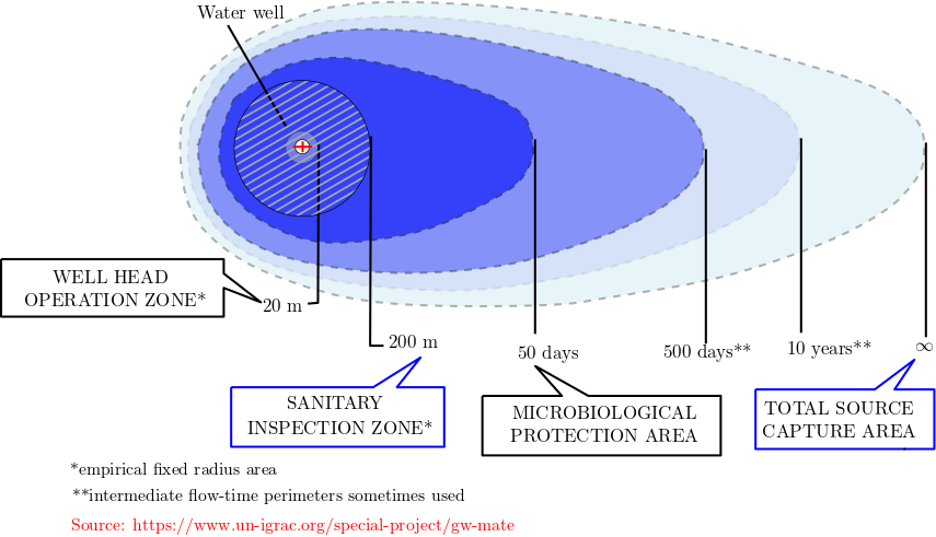
Fig. 5.14 A schematic of the groundwater protection zone.#
As can be observed in the figure, the zones are based on the travel time, and each travel time is divided into protection of groundwater resources against different activities.
In Germany law DVGW W-101 exitst for groundwater protection zones. As per the German rule, the groundwater protection zones is divided into three different zones:
Zone I : The immediate protection zone - at least 10 m from the water well, not less than 20 m in the upstream direction of a spring.
Zone II : The inner protection zone - 50-day travel time but not less than 100 m from the well or spring.
Zone III : The outer protection zone - entire contribution zone of the groundwater catchment area (maybe sub-divided see figure)
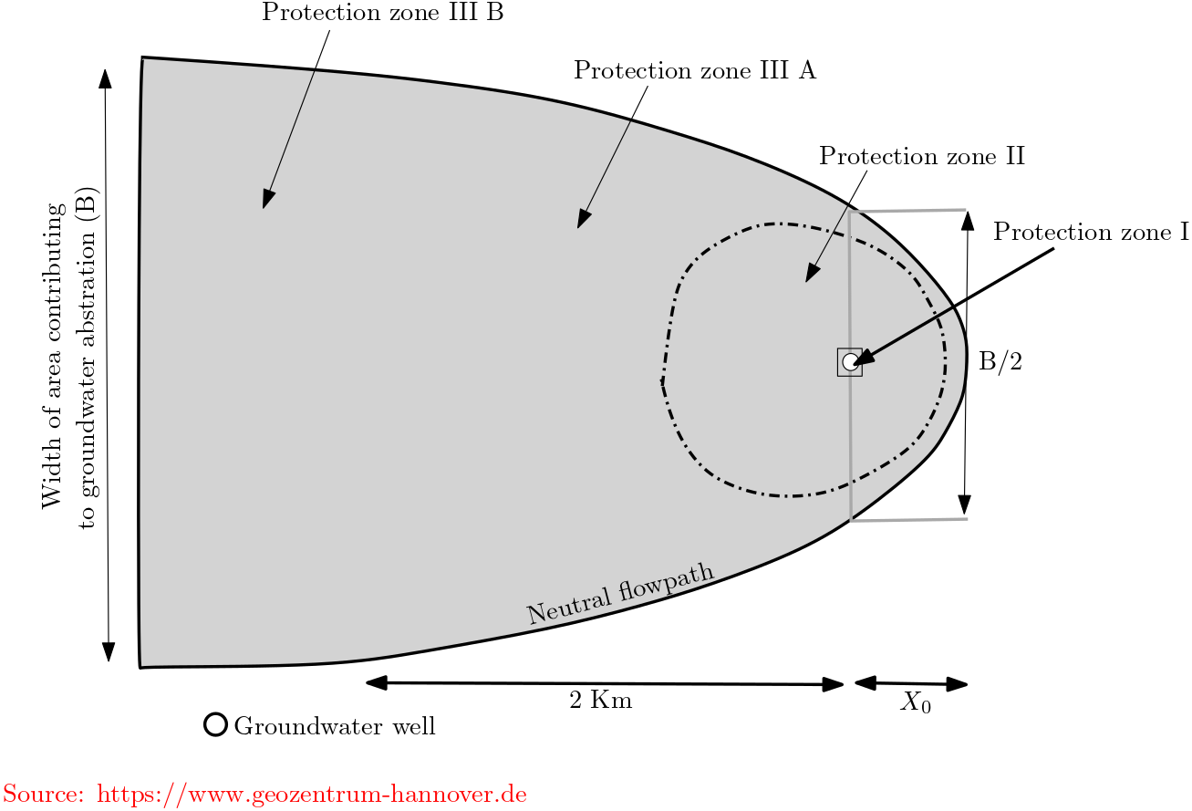
Fig. 5.15 Groundwater protection zone in Germany#
5.7.3. Well Capture Zones in Natural Aquifers#
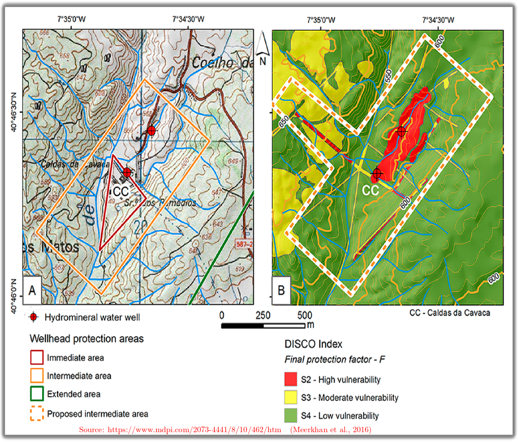
Fig. 5.16 Groundwater protection zone natural aquifers#
5.8. Darcy’s Law in Anisotropic#
5.8.1. Principal Axes of Hydraulic Conductivity#
In anisotropic aquifer refers to those aquifers whose properties vary with direction. This means that properties such as hydraulic conductivity will have maximum value along a direction and the minimum value along the other direction. It has been found that (also depicted in fig :refnum:`axes_an`) these two directions are perpendicular to each other. This is true in general, not only for the layered systems that was covered in the previous lecture
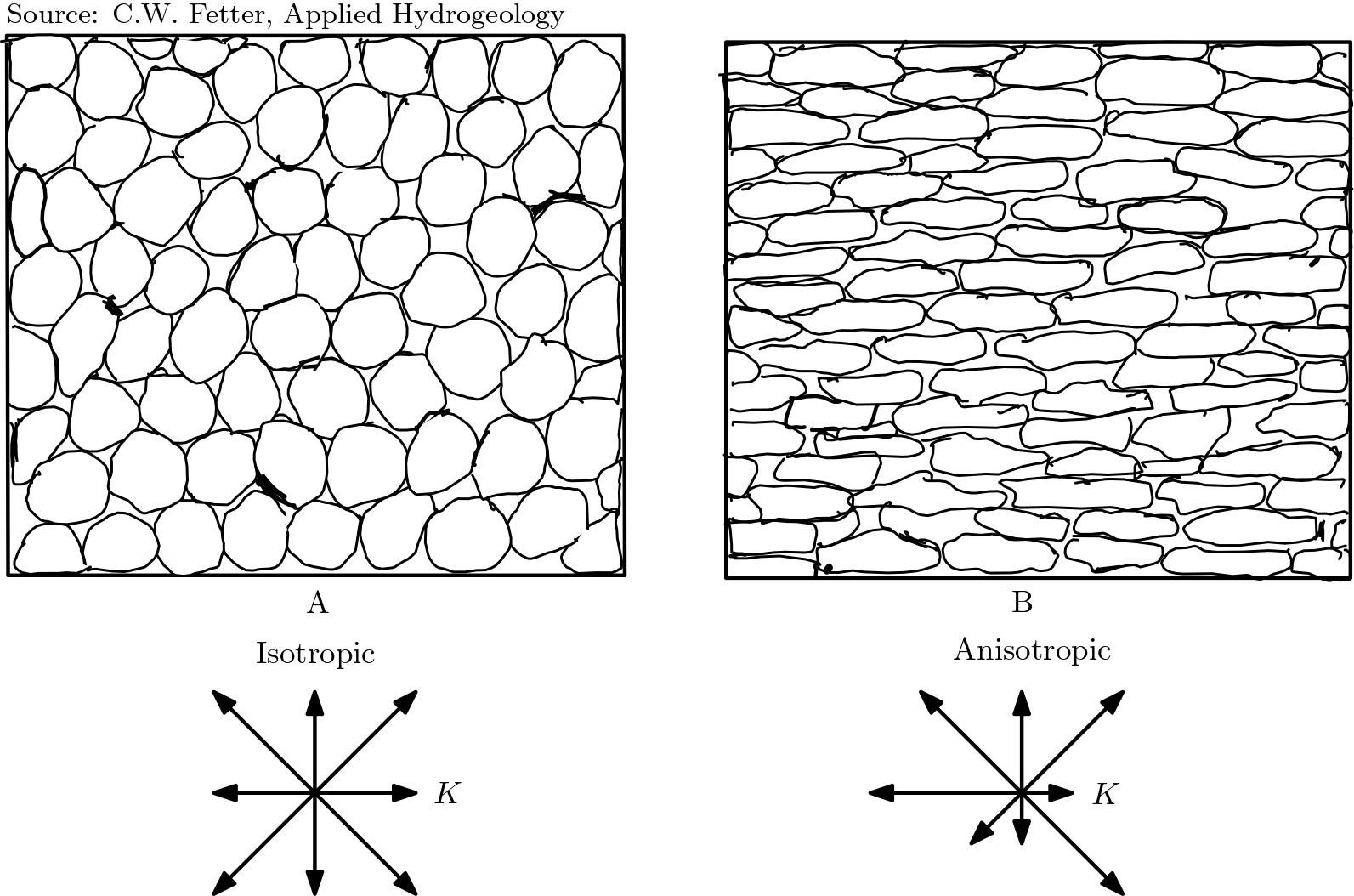
Fig. 5.17 Hydraulic conductivity in anisotropic aquifers#
The three principal axes of hydraulic conductivity are oriented
along the direction with maximum hydraulic conductivity
along the direction with hydraulic conductivity
perpendicular to both
5.8.2. Formulation of Darcy’s Law in Anisotropic Aquifers#
If the principal axes of conductivity coincide with the axes of a Cartesian coordinate system, Darcy’s law for anisotropic aquifer is given as
In this equation, hydraulic conductivity has to be written as a matrix. To be precise, \(K\) represents a tensor, i.e., a quantity which is subject to certain rules under coordinate transforms (from Cartesian to cylinder coordinates, for example). These rules guarantee that Darcy’s law can also be applied in coordinate systems other than Cartesian.
If the aquifer is isotropic in the horizontally oriented \(xy\)-plane, we get,
The most general case is encountered when all principal axes are associated with different hydraulic conductivities and none of them coincides with a coordinate axis:
From this, one may easily conclude that it is advantageous to arrange coordinate axes in parallel with principal axes of \(K\). Unfortunately, this is not always possible, e.g., when layers are folded.
5.8.3. Direction of flow#
With directional dependence on conductivity also affects the direction of the flow. This is summarized in the figure below. Basically we have
Isotropic aquifer: \(K\) can be represented by a scalar and the direction of flow is opposite to the direction of the gradient.
Anisotropic aquifer: \(K\) has to be represented by a tensor (matrix) and the angle between the gradient vector and the flow direction is between 90° and 180°.

Fig. 5.18 Direction of flow in anisotropic aquifer#
5.8.4. Examples for Flow Nets in Anisotropic Aquifers#
The figure provides flow nets for different ratios of anisotropy but for the identical conditions at domain boundaries (i.e., inflow from the top, outflow to a pipe on the left). As can be observed isolines and streamlines intersect each other at right angles only if the aquifer is isotropic.
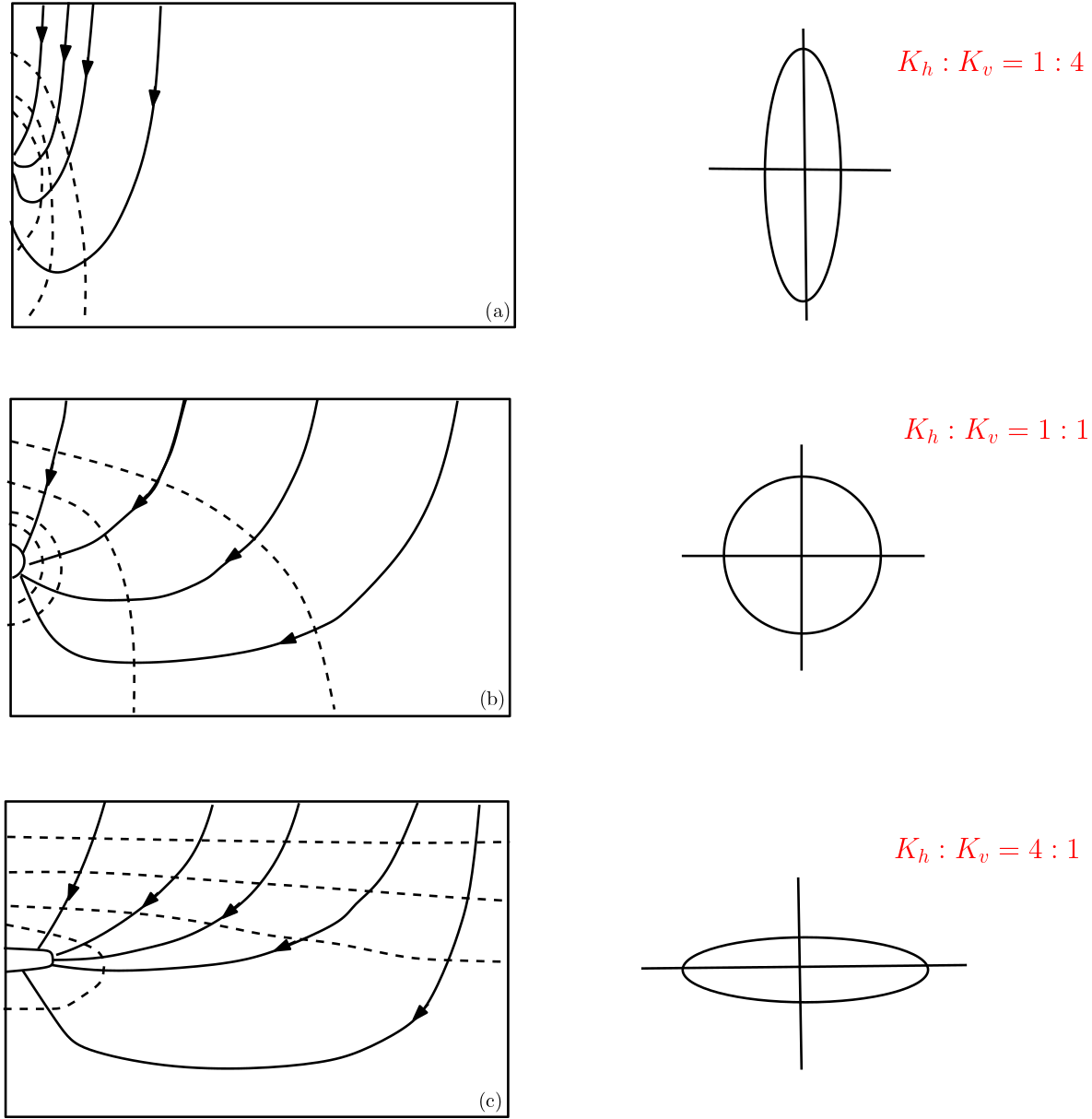
Fig. 5.19 Flow nets in anisotropic aquifer#
The interactive simulation on effect of anisotropy on flux and gradient can be found in: Tools Section as Simulating Anisotropy and Flow Direction
# The library used

import numpy as np
import matplotlib.pyplot as plt
import pandas as pd
from ipywidgets import widgets, interactive


# the main programme
def aniso(a_d, ani_r):

# interim calculation
    a_r = a_d*np.pi/180

    i_xr = np.cos(a_r) # (-), rel. hyd grad. along x
    i_zr = np.sin(a_r) # (-), rel. hyd grad. along z
    K_h = 1 # (-), m/s K_h
    K_v = 1/ani_r # m/s, rel K_v
    f_x = -i_xr*K_h # m/s
    f_z = -i_zr*K_v # m/s
    f_m = np.sqrt(f_x*f_x+f_z*f_z) # m/s

    args = (K_h*i_xr*i_xr + K_v*i_zr*i_zr)/f_m
    an_i_f = ((np.pi-np.arccos(args))*180/np.pi)# deg,

# plots axes

    fig, (ax1, ax2) = plt.subplots(1, 2,figsize=(10,6), gridspec_kw={'width_ratios': [3, 1]})

# points for gradient and flux

    grad_px = [0, i_xr]#i_xr
    grad_pz = [0, i_zr]#i_zr

    flux_px = [0, f_x]
    flux_pz = [0, f_z]

# creating points for intersect lines (5 of them)

    p1=-0.5*i_zr; p2 = 0.5*i_zr; p3 =-0.5*i_zr+0.35*i_xr; p4 = 0.5*i_zr+0.35*i_xr; p5 = -0.5*i_zr+0.7*i_xr
    p6 = 0.5*i_zr+0.7*i_xr;p7 = -0.5*i_zr-0.35*i_xr; p8 = 0.5*i_zr-0.35*i_xr; p9 = -0.5*i_zr-0.7*i_xr;p10 =0.5*i_zr-0.7*i_xr

    q1=0.5*i_xr; q2 =- 0.5*i_xr; q3 =0.5*i_xr+0.35*i_zr; q4 = -0.5*i_xr+0.35*i_zr; q5 = 0.5*i_xr+0.7*i_zr
    q6 = -0.5*i_xr+0.7*i_zr;q7 = 0.5*i_xr-0.35*i_zr;q8 = -0.5*i_xr-0.35*i_zr; q9 = 0.5*i_xr-0.7*i_zr;q10 = -0.5*i_xr-0.7*i_zr

# plotted points
    l_1x =[p1, p2]; l_1y = [q1, q2]
    l_2x =[p3, p4]; l_2y = [q3, q4]
    l_3x =[p5, p6]; l_3y = [q5, q6]
    l_4x =[p7, p8]; l_4y = [q7, q8]
    l_5x =[p9, p10]; l_5y = [q9, q10]


# creating points for anisotropy
    r1 =1.05 if ani_r >= 1 else 1.5-0.45*ani_r
    r2 = 1.95 if ani_r >= 1 else 1.5+0.45*ani_r
    r3 = 0.5*(r1+r2); r4 = r3

    s1 = -0.5; s2 = s1
    s3 = -0.05 if ani_r<=1 else -0.5+0.45/ani_r
    s4 = -0.95 if ani_r<=1 else -0.5-0.45/ani_r

# plotted points
    Iso_1x = [r1, r2]; Iso_1y = [s1, s2]
    Iso_2x = [r3, r4]; Iso_2y = [s3, s4]
    Iso_x =[r1, r2, r3, r4]; Iso_y = [s1,s2,s3,s4]

# plotting all points

# plotting gradient/flux lines

    ax1.plot(grad_px, grad_pz, "g", label=" gradient") # plotting gradient
    ax1.plot(flux_px, flux_pz, "r", label=" flux") # plotting flux

# plotting intersect lines
    ax1.plot(l_1x, l_1y, "b", label = "head isoline")
    ax1.plot(l_2x, l_2y, "b")
    ax1.plot(l_3x, l_3y, "b")
    ax1.plot(l_4x, l_4y, "b")
    ax1.plot(l_5x, l_5y, "b")
    ax1.legend()


    ax1.spines['left'].set_position('center') # bring the axis lines in center
    ax1.spines['bottom'].set_position('center')
    ax1.spines['right'].set_color('none') # remove the top box
    ax1.spines['top'].set_color('none')
    ax1.set_xticks([]);ax1.set_yticks([]); # remove the ticks
    ax1.set_title("Anisotropy flux and gradient", y=0, pad=-25, verticalalignment="top")


# plotting Anisotropy
    ax2.plot(Iso_1x, Iso_1y, "k", label = r"$K_h: K_v$")
    ax2.plot(Iso_2x, Iso_2y, "k")
    ax2.legend(bbox_to_anchor=(-0.4, -0.05), loc='lower left')
    ax2.set_xlim(1, 2)
    ax2.set_ylim(-1, 1)
    ax2.axis('off')
    ax2.set_title("Anisotropy ratio", y=0, pad=-25, verticalalignment="top");

interactive(aniso,
         a_d=widgets.BoundedFloatText(value=45, min=0, max=360, step=0.5, description=r'angle (°)', disabled=False),
         ani_r=widgets.BoundedIntText(value=1, min=1, max=100, step=1, description='K<sub>h</sub>/K<sub>v</sub>', disabled=False),)
