9. Simulating 1D Trench Flow

The tool simulates the effect on the water table due to model parameters.

Contributed by Ms. Anne Pförtner and Sophie Pförtner. The original concept from Prof. R. Liedl spreasheet code.

9.1. Scenario and Equation

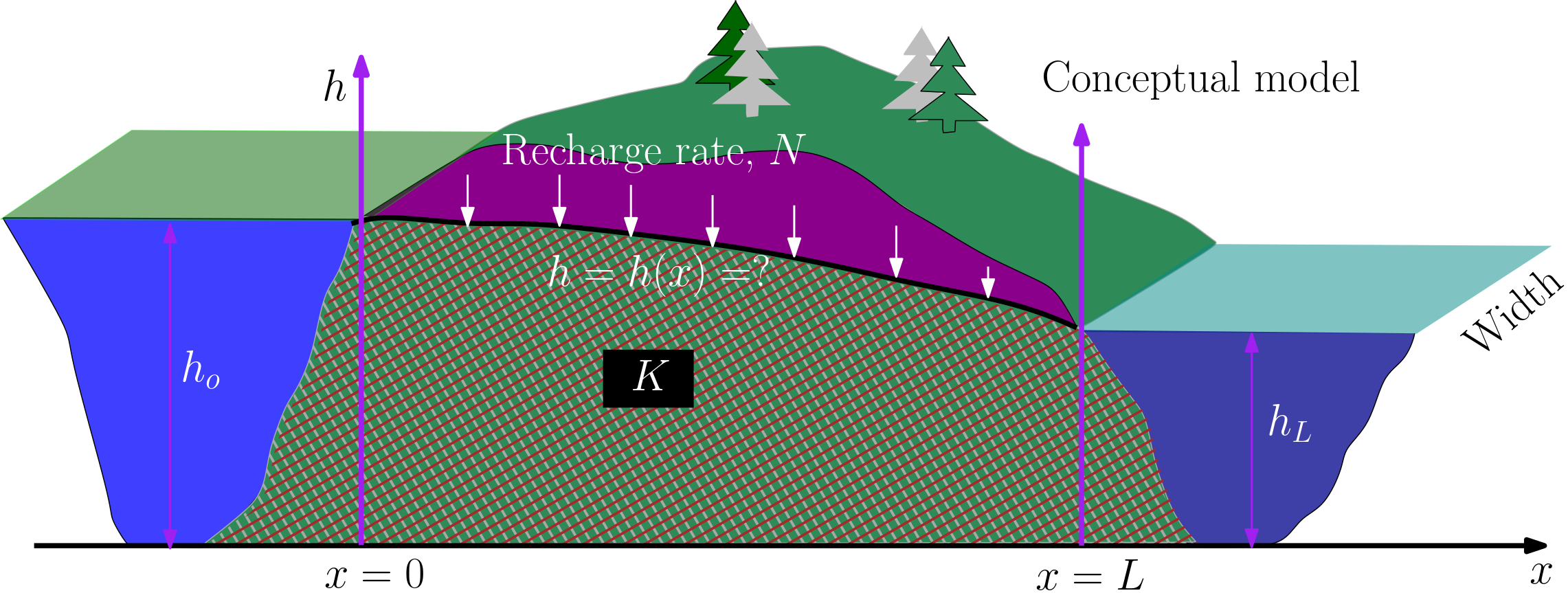
Fig. 9.1 Conceptual model of a flow between two water bodies separated by unconfined aquifer

You can calculate the steady flow in an unconfined aquifer with this Equations¹ :

\[q' = \frac{1}{2} \cdot K \cdot \frac{H_o^2-H_u^2}{L}\]

\[h(x)=\sqrt{H_o^2 - \frac{H_o^2-H_u^2}{L} \cdot x+\frac{R}{K} \cdot x \cdot(L-x)}\]

with
\(q'\) = flow per unit width \([m^2/s]\), \(h\) = head at x \([m]\),
\(x\) = distance from the origin \([m]\), \(H_o\) = head at the origin \([m]\), \(H_u\) = head at L \([m]\), \(L\) = distance from the origin at the point \(H_u\) is measured \([m]\), \(K\) = hydraulic conductivity \([m/s]\), \(R\) = recharge rate \([m/s]\)

9.1.1. How to use this tool

1. Go to the Binder by clicking the rocket button (top-right of the page)

2. Execute the code cell with libraries and the code cell

3. Interact with the sliders.

This tool can also be downloaded and run locally. For that download the 1D_ditchflow.ipynb file from the book GitHub site, and execute the process in any editor (e.g., JUPYTER notebook, JUPYTER lab) that is able to read and execute this file-type.

The codes are licensed under CC by 4.0 (use anyways, but acknowledge the original work)

# Initialize librarys
import matplotlib.pyplot as plt
import numpy as np
import math
from ipywidgets import *

# Definition of the function
def head(Ho, Hu, L, R, K):

    """
    Ho: inflow head in [m]
    Hu: outflow head in [m]
    L:  Domain length in [m]
    R:  Recharge rate in [mm/d]
    K: Hydraulic conductivity in [m/s]
    """
    x = np.arange(0, L,L/1000)
    R=R/1000/365.25/86400
    h=(Ho**2-(Ho**2-Hu**2)/L*x+(R/K*x*(L-x)))**0.5
    plt.plot(x, h)
    plt.ylabel('head [m]')
    plt.ylim(0,1.5*Ho)
    plt.xlabel('x [m]')
    plt.xlim(0,L)
    plt.show()

style = {'description_width': 'initial'}  
interact(head,
         Ho=widgets.BoundedFloatText(value=10, min=0, max=1000, step=0.1, description='Ho:', disabled=False),
         Hu=widgets.BoundedFloatText(value=7.5, min=0, max=1000, step=0.1, description='Hu:', disabled=False),
         L= widgets.BoundedFloatText(value=175,min=0, max=10000,step=1, description='L:' , disabled=False),
         R=(-500,2500,10),
         K=widgets.FloatLogSlider(value=0.0002,base=10,min=-6, max=-2, step=0.0001,readout_format='.2e'))

<function __main__.head(Ho, Hu, L, R, K)>

---

1

C. W. Fetter, Thomas Boving, David Kreamer (2017), Contaminant Hydrogeology: Third Edition, Waveland Press