Darcy Law and Conductivity
Contents
import numpy as np
import matplotlib.pyplot as plt
import pandas as pd
import panel as pn
pn.extension("katex")
4. Darcy Law and Conductivity#
(The contents presented in this section were re-developed principally by Dr. P. K. Yadav. The original contents are from Prof. Rudolf Liedl)
tutorial problems on Darcy’s law and intrinsic permeability
homework problems on Darcy’s law and intrinsic permeability
4.1. Tutorial Problems on#
Darcy’s Law and
Intrinsic Permeability
4.2. Tutorial Problem 7: Flow Direction and Hydraulic Gradient#
Indicate the direction of flow shown in the figure in next slides, and determine the hydraulic gradient for a Darcy column with length L = 50 cm! (Figures not to scale.)
4.2.1. Tutorial Problem 7 – Solution#
The relevant topic is covered in Lecture 04, slide 8
# Image (a)
L = 0.5 # m, length of the column
Ea_hl = 0.2 #, m, elevation head, left
Pa_hl = 0.1 #, m  pressure head, left
Ea_hr = 0.2 #, m, elevation head, right
Pa_hr = 0.3 #, m  pressure head, right
Ha_hl = Ea_hl + Pa_hl # m, hydraulic head, left
Ha_hr = Ea_hr + Pa_hr # m, hydraulic head, right
DH_a = Ha_hr - Ha_hl
H_ga = DH_a/L#, no unit, hydraulic gradient

print("Hydraulic head LEFT: {0:1.1f}".format(Ha_hl),"m"); print("Hydraulic head RIGHT:: {0:1.1f}".format(Ha_hr),"m")
print("Hydraulic Head Difference: {0:1.1f}".format(DH_a),"m");print("Hydraulic gradient: {0:1.1f}".format(H_ga))
png_pane.object = "images/T03_TP7_a2.png"
Hydraulic head LEFT: 0.3 m
Hydraulic head RIGHT:: 0.5 m
Hydraulic Head Difference: 0.2 m
Hydraulic gradient: 0.4
# Image (b)
L = 0.5 # m, length of the column
Eb_hl = 0.2 #, m, elevation head, left
Pb_hl = 0.1 #, m  pressure head, left
Eb_hr = 0.05 #, m, elevation head, right
Pb_hr = 1.3 #, m  pressure head, right
Hb_hl = Eb_hl + Pb_hl # m, hydraulic head, left
Hb_hr = Eb_hr + Pb_hr # m, hydraulic head, right
DH_b = Hb_hr - Hb_hl
H_gb = DH_b/L#, no unit, hydraulic gradient
print("Hydraulic head LEFT: {0:1.1f}".format(Hb_hl),"m");print("Hydraulic head RIGHT:: {0:1.1f}".format(Hb_hr),"m")
print("Hydraulic Head Difference: {0:1.1f}".format(DH_b),"m");print("Hydraulic gradient: {0:1.1f}".format(H_gb))
png_pane2.object = "images/T03_TP7_b2.png"
Hydraulic head LEFT: 0.3 m
Hydraulic head RIGHT:: 1.4 m
Hydraulic Head Difference: 1.1 m
Hydraulic gradient: 2.1
# Image (c)
L = 0.5 # m, length of the column
Ec_hl = 0.3 #, m, elevation head, left
Pc_hl = 0.1 #, m  pressure head, left
Ec_hr = 0.2 #, m, elevation head, right
Pc_hr = 0.2 #, m  pressure head, right
Hc_hl = Ec_hl + Pc_hl # m, hydraulic head, left
Hc_hr = Ec_hr + Pc_hr # m, hydraulic head, right
DH_c = Hc_hr - Hc_hl
H_gc = DH_c/L#, no unit, hydraulic gradient
print("Hydraulic head LEFT: {0:1.1f}".format(Hc_hl),"m");print("Hydraulic head RIGHT:: {0:1.1f}".format(Hc_hr),"m")
print("Hydraulic Head Difference: {0:1.1f}".format(DH_c),"m");print("Hydraulic gradient: {0:1.1f}".format(H_gc))
png_pane3.object = "images/T03_TP7_c2.png"
Hydraulic head LEFT: 0.4 m
Hydraulic head RIGHT:: 0.4 m
Hydraulic Head Difference: 0.0 m
Hydraulic gradient: 0.0
# Image (d)
L = 0.5 # m, length of the column
Ed_hl = 0.3 #, m, elevation head, left
Pd_hl = 0.1 #, m  pressure head, left
Ed_hr = 0.2 #, m, elevation head, right
Pd_hr = 0.1 #, m  pressure head, right
Hd_hl = Ed_hl + Pd_hl # m, hydraulic head, left
Hd_hr = Ed_hr + Pd_hr # m, hydraulic head, right
DH_d = Hd_hr - Hd_hl
H_gd = DH_d/L#, no unit, hydraulic gradient
#output
print("Hydraulic head LEFT: {0:1.1f}".format(Hd_hl),"m");print("Hydraulic head Right:: {0:1.1f}".format(Hd_hr),"m")
print("Hydraulic Head Difference: {0:1.1f}".format(DH_d),"m");print("Hydraulic gradient: {0:1.1f}".format(H_gd))
png_pane4.object = "images/T03_TP7_d2.png"
Hydraulic head LEFT: 0.4 m
Hydraulic head Right:: 0.3 m
Hydraulic Head Difference: -0.1 m
Hydraulic gradient: -0.2
4.3. Tutorial Problem 8#
The hydraulic conductivity of a fine sand sample was found to be equal to \(1.36\times 10^{-5}\) m/s in a Darcy experiment using water at a temperature of \(20^\circ\)C. What is the intrinsic permeability of this sample? Give results in cm\(^2\) and D. (density of water at \(20^\circ\)C: 998.2 kg/m\(^3\); dynamic viscosity of water at \(20^\circ\)C: \(1.0087 \times 10^{-3}\) Pa\(\cdot\)s; 1 D = \(0.987\times 10^{-12}\) m\(^2\))
4.3.1. Tutorial Problem 8 - Solution#
Relevant topics are covered in Lecture 04 slides 18-20.
Relationship between hydraulic conductivity \(K\) and intrinsic permeability \(k\) from lecture notes: $\( K_{water} = k\cdot \frac{\rho_{water}\cdot g}{\eta_{water}} \)$
Solve for , \(k\)
#Given
Darcy = 0.987 * 10**-12 # m^2, 1D = 0.987*10^-12 m^2
nu_w = 1.00087*10**-3 # Pa-S dynamic viscosity of water
K_w = 1.36*10**-5 # m/s Conductivity of water
g = 9.81 # m/s^2 accln due to gravity
rho_w = 998.2 # kg/m^3, density of water

# Solution
k = (nu_w*K_w)/(rho_w*g)#, m^2, permeability of water
k_D = k/Darcy


print("The permeability is {0:1.1E}".format(k),"m\u00b2")
print("The permeability in Darcy unite is: {0:1.2f}".format(k_D),"D")
The permeability is 1.4E-12 m²
The permeability in Darcy unite is: 1.41 D
4.4. Tutorial Problem 9: Constant-Head Permeameter#
#Given (solution on 9b)
L = 15 #cm, length of column
A = 25 # cm^2, surface area of column
h_diff = 5 # cm, h_in-h_out
Q = 100/12 # cm^3/min discharge per min

# Solution using derived equation in first part of the problem
# K = QL/A(h_in- h_out)

K = (Q*L)/(A*h_diff)# cm/min, required conductivity
K_1 = K*10**-2/60 #, m/s, conductivity in m/s

#output
print("The conductivity in column is {0:1.2E}".format(K),"cm/min")
print("The conductivity in column is {0:1.2E}".format(K_1),"m/s \n")

if K_1 <= 1.67*10**-4:
    print("Fine to medium sand")
else:
    print("to check further") # to be completed later.
The conductivity in column is 1.00E+00 cm/min
The conductivity in column is 1.67E-04 m/s

Fine to medium sand
Continue solution on 9c
Discharge and Darcy’s law: \(Q_{water} = \frac{V}{t_{water}}=-A\cdot K_{water}\cdot\frac{\Delta h}{L}\)
Solve for \(t_{water}\): \(t_{water} = \frac{V}{Q_{water}}=-\frac{V}{A\cdot K_{water}\cdot\Delta h/L} = -\frac{V\cdot L}{A\cdot K_{water}\cdot\Delta h}\)
Same step for \(t_{diesel}\): \(t_{diesel} = -\frac{V\cdot L}{A\cdot K_{diesel}\cdot\Delta h}\)
time ratio:\(\frac{t_{diesel}}{t_{water}} = \frac{-\frac{V\cdot L}{A\cdot K_{diesel}\cdot\Delta h}}{-\frac{V\cdot L}{A\cdot K_{water}\cdot\Delta h}} = \frac{K_{water}}{K_{diesel}}\)
Use relationship between conductivity \(K\) and permeability \(k\) from lecture notes (slides 18) $\(\frac{K_{water}}{K_{diesel}} = \frac{k\cdot \frac{\rho_{water}\cdot g}{\eta_{water}}}{k\cdot \frac{\rho_{diesel}\cdot g}{\eta_{diesel}}} = \frac{\rho_{water}\cdot\eta_{diesel}}{\rho_{diesel}\cdot\eta_{water}}\)$
Solve for \(t_{diesel}\)
# Given data

rho_w = 920.2 # kg/m^3, density of water at 20°C
eta_w = 1.0087*10**-3#, Pa-S dynamic viscosity of water
rho_d = 0.85 # g/cm^3, density of diesel at 20°C
eta_d = 3.5*10**-3#, Pa-S dynamic viscosity of diesel
V_d = 100 # cm^3 volume of diesel
t_w = 12 # min, time taken by water

# Calculations

t_d = (rho_w*eta_d)/(rho_d*1000*eta_w)*t_w

# multiplied by 1000 to convert unit g/cm^3 to kg/m^3

print("The time required for diesel will be: {0:0.2f}".format(t_d), "min")
The time required for diesel will be: 45.08 min
4.5. Tutorial Problem 10: Falling-Head Permeameter#
# Solution 9(2)

L = 15 # cm, length
L_m = L/100 # m, length
d_c = 10 # cm, diameter column
d_t = 2 # cm, diameter tube
h_d0 = 5 # cm, head difference at start
h_dt = 0.5 # cm, head difference at time t
t = 528 # min, total time
t_s = 528*60 # sec, total time in seconds

#solution using the developed equation

K = (d_t/d_c)**2 * ((L_m)/t_s)*np.log(h_d0/h_dt)

#Output
print("The conductivity in column is {0:1.2E}".format(K),"m/s \n")

if K < 1.67*10**-5:
    print("Silt or silty sand")
else:
    print("to check further") # to be completed later.
The conductivity in column is 4.36E-07 m/s

Silt or silty sand
4.6. HOME WORK PROBLEMS#
Darcy’s Law and Intrinsic Permeability
There is no obligation to solve homework problems!
Try to submit within next 2 weeks.
4.7. Homework Problem 3#
4.8. Homework Problem 4#
#
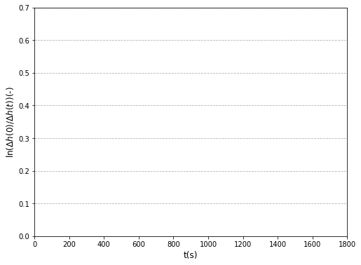
fig, ax = plt.subplots(figsize=(8, 6))
plt.grid(axis='y', linestyle='--')
plt.xlim((0, 1800)); plt.ylim((0,0.7))
plt.xlabel("t(s)", fontsize=12 )
plt.ylabel(r"ln($\Delta h(0)/\Delta h(t)$)(-)", fontsize=12);


