Conservative transport
Contents
import numpy as np
import matplotlib.pyplot as plt
import pandas as pd
import panel as pn
pn.extension('katex')
9. Conservative transport#
Solution of Homework Problems 8 - 9
Tutorial Problems on Conservative Transport
Homework Problems on Conservative Transport
9.1. Homework Problem 8: Flow in confined aquifer#
rh8_1 = pn.pane.LaTeX(r"""
Presented below in the figure is the available information of an aquifer cross-section.
The aquifer is confined and of variable thickness across the cross-section. It has a uniform conductivity
$5.6 \times 10^{-5}$ m/s. The total Discharge from the aquifer of width 500 m is required to be obtained.
""",width = 400, style={'font-size': '12pt'})

rh8_2 = pn.pane.PNG("images/T06_HP8.png", width=500)

pn.Row(rh8_1, rh8_2)
9.1.1. Solution Homework Problem 8#
#solution Homework problem 8

rh8_3 = pn.pane.LaTeX(r"""
The aquifer is confined but of variable thickness, hence $T = Kb$, cannot be used. In this case we need to
find a representative aquifer thickness. This is simple if it can be assumed that a slope decreases linearly through-out
its length. So, we can write for a representative $m$
$$
m = \frac{m_3-m_1}{L}x + m_1  \qquad\qquad \text{(eq. 2A)}
$$
where $x$ is a lengthwise distance of $m$ from $m_1$. Equation above is simply
an equation of straight line $y = ax + c$, in which slope $a = \frac{m_3-m_1}{L} $ and $c = m_1$.

Now Darcy law can be used to obtain discharge per unit width ($q'$).

$$
q' = -mK\frac{dh}{dx} \qquad\qquad \text{(eq. 2B)}
$$

with conductivity $K$ and hydraulic head gradient $dh/dx$. We substitute $b$ from eq. (2A) to eq. (2B)
$$
q' = -\Bigg(\frac{m_3-m_1}{L}x + m_1\Bigg) \cdot K\frac{dh}{dx}  \qquad\qquad \text{(eq. 2C)}
$$

Rearranging eq. (2C) we get
$$
-dh = \frac{q'}{K}\cdot \frac{dx}{\frac{m_3 - m_1}{L}x+m_1}
\qquad\qquad \text{(eq. 2D)}
$$

Differential equation Eq. (2D) has to be solved to obtain the discharge.

""",width = 900, style={'font-size': '13pt'})
rh8_3
#Homework problem 8 – Continued

rh8_4 = pn.pane.LaTeX(r"""
Eq. (2D) is a variable separated differential equation, so direct integration can be done with the following hydraulic (boundary) conditions:
$$
\text{for } x = 0,  \; h = h_1 \qquad \text{and}\qquad \text{for } x = L, \; h = h_3
$$

i.e.,
$$
-\int_{h_1}^{h_3} dh = \frac{q'}{K}\cdot\int_0^L \frac{dx}{\frac{m_3-m_1}{L}x + m_1}
\qquad \qquad \text{eq. (2E)}$$

The integral on the right hand side of eq. (2E) is an elementary integral the solution of which is of the form:
$$
\int\frac{dx}{ax + b} = \frac{1}{a}\ln(ax+b) + C
$$
based on this, the solution of eq. (2E) will be
$$
h_1 - h_3 = \frac{q'}{K} \frac{1}{\frac{m_3-m_1}{L}}\cdot\Bigg[\ln\Bigg(\frac{m_3-m_1}{L}L + m_1 \Bigg) - \ln\Bigg(\frac{m_3-m_1}{0}0 + m_1 \Bigg)\Bigg]
$$
Simplifying which we get
$$
h_1 - h_3  = \frac{q'}{K}\cdot \frac{L}{m_3-m_1}\cdot \ln\frac{m_3}{m_1}
$$
Then, $q'$ the unit aquifer width discharge can be obtained from
$$
q' = K \frac{h_1- h_3}{L}\cdot\frac{m_3 - m_1}{\ln\frac{m_3}{m_1}}
\qquad \qquad \text{eq. (2F)}$$
""",width = 900, style={'font-size': '13pt'})
rh8_4
#Homework Problem 8 – Continued
# given
h8_1 = 290 # m, head in Well 1
h8_3 = 275 # m, head in the river end
m8_1 = 6 # m, aquifer thickness at well 1
m8_3 = 20 # m, aquifer thickness near river end
K8 = 5.6 * 10**-6 # m/s, conductivity of aquifer
L8 = 700 # m, length of the river cross-section
W8 = 500 # m, Width of aquifer

# solution
# Discharge per unit width using eq. 2F
q8 = K8*((h8_1 - h8_3)/L8)*(m8_3 - m8_1)/np.log(m8_3/m8_1)
Q8 = q8*W8

#output
print("Discharge per unit width of aquifer is: {0:1.2e}".format(q8), "m\u00b2/s \n")
print("Discharge from the given width of aquifer is: {0:1.2e}".format(Q8), "m\u00b3/s")
Discharge per unit width of aquifer is: 1.40e-06 m²/s

Discharge from the given width of aquifer is: 6.98e-04 m³/s
9.1.2. Homework Problem 9 - Unconfined aquifer#
rh9_1 = pn.pane.LaTeX(r"""
In a schematic below an unconfined aquifer is found to divide 2 rivers of differnt stages $h_1 = 30$ m and $h_2 = 10$ m.
The aquifer of length $L = 50$ m and with uniform conductivity $K = 5\times 10^{-6}$ m/s is found to receive recharge at
the rate ($w$) of 0.01 m/d. <br>
a) What will be the hydraulic head and discharge per unit width ($q'$) in the aquifer at 5 m
from the left river. <br>
b) What will the head at the same location when aquifer receives no recharge.

""",width = 900, style={'font-size': '12pt'})

rh9_2 = pn.pane.PNG("images/T06_HP9.png", width=450)

pn.Column(rh9_1, rh9_2)
9.1.3. Solution of Homework Problem 9#
# Solution of Homework Problem 9

rh9_3 = pn.pane.LaTeX(r"""

For an unconfined aquifer, the case here, the water table = hydraulic head. For a condition as in this problem the height
of the water table $h$ as a function of position $x$ can be obtained from the following expression provided in Fetter (2014):
$$
h = \sqrt{h_1^2 - \frac{(h_1^2- h_2^2)x}{L} + \frac{w}{K}(L-x)x}
\quad\quad \text{eq. (3A)}
$$

From which discharge per unit width $(q')$ can be obtained by differentiating eq. (3A) with respect to $x$,
and using Darcy Law $q' = -Kh (dh/dx)$ for unconfined aquifer. Fetter (2014) provides the following solution:
$$
q'(x) = \frac{K (h_1^2 - h_2^2)}{2L}- w\Bigg(\frac{L}{2}-x\Bigg)
\quad\quad \text{eq. (3B)} $$

For the case when $w= 0$, the last term under the square root in eq. (3A) becomes 0, and then $h$ is
$$
h = \sqrt{h_1^2 - \frac{(h_1^2- h_2^2)x}{L}}
\quad\quad \text{eq. (3C)}
$$

""",width = 900, style={'font-size': '13pt'})


rh9_3
#Solution of Homework Problem 9
# Given

h9_1 = 30 # m, River 1 stage
h9_2 = 10 # m, River 2 stage
K9 = 5 * 10**-4 # m/s uniform conductivity of aquifer
L9 = 50 # m, length of the aquifer
w9 = 0.01/(24*3600) # m/s recharge rate in the aquifer
x9 = 5 # m, loaction at which water table is to be found

#Calculation part a
h9_w = np.sqrt(h9_1**2 - ((h9_1**2 - h9_2**2)*x9)/L9 + (w9/K9)*(L9-x9)*x9) # head at x = 5 m from eq. 4A
q9 = K9*((h9_1**2- h9_2**2)/2*L9) - w9*((L9/2)-x9)     # m^2/s, total dischage from given width

#Calculation part b
h9_nw = np.sqrt(h9_1**2 - ((h9_1**2 - h9_2**2)*x9)/L9)


#output
print("The water table at the required  location (x) with recharge is: {0:1.5f}".format(h9_w), "m \n")
print("Discharge per unit width from the aquifer is: {0:1.2f}".format(q9), "m\u00b2/s \n")
print("The water table at the required  location (x) without recharge is: {0:1.5f}".format(h9_nw), "m ")
The water table at the required  location (x) with recharge is: 28.63655 m

Discharge per unit width from the aquifer is: 10.00 m²/s

The water table at the required  location (x) without recharge is: 28.63564 m
9.1.4. Tutorial Problem 20#
A column (\(L = 1\) m and \(\oslash= 5\) cm) was packed with sandy soil (\(n_e= 35\%\), \(K= 0.0002\) m/s). The hydraulic head at the inlet and the outlet was set to 235 m and 230 m, respectively. The NaCl solution with concentration 10 mg/L was steadily introduced to the column after saturating it with distilled water. The experiment condition was such that the diffusive flow could be neglected.
A. Determine the advective mass flow and the mass flux entering the column?
B. What will be the concentration at the outlet of the column when only advective flow is considered? Consider the NaCl conc. = 0 at the outlet initially.
C. What will be the dispersion coefficient assuming dispersivity is 0.001 m?
9.1.5. Solution of Tutorial Problem 20#
# Solution Tutorial Problem 20 A.

# Given are:

L = 1 # m, length of tube
n_e = 0.35 # (-), effective porosity
C = 10 # mg/L , NaCl concentration
d = 5 # cm, diameter of pipe
K = 0.0002 # m/s, conductivity
hin = 230 # m, head inlet
hout = 235 # m, head outlet

# intermediate problem
d_m = d/100 # m, diameter in m
C_k = C/1000 # kg/m³ conc. unit change
A_c = np.pi/4*(d_m)**2 # m², area column
dh = (hout-hin) # m, head difference
hd = dh/L
v = (K*dh/L)/n_e # m/s velocity = q/ne= (K*dh/L)/n_e

# calculation and print out
J_adv = n_e*v*A_c*C_k # Kg/s, advective flow
j_adv = J_adv/A_c # Kg/(m^2-s), advective flux

print('\033[1m Results are:\033[0m \n')
print("The required advective mass flow is{0:0.2f}".format(J_adv), "Kg/s \n")
print("The required advective mass flow is{0:0.2f}".format(J_adv), "Kg/m\u00b2-s")
 Results are:

The required advective mass flow is0.00 Kg/s

The required advective mass flow is0.00 Kg/m²-s
Solution Tutorial Problem 20 B.
If only advective flow is considered, i.e., dispersion and diffusion is not present and we get:
Integrating the equation between \(C_{in}\) and \(C_{out}\), we get
The concentration at the outlet = inlet = 10 mg/L.
# solution Tutorial Problem 20 C.

# Given

dy = 0.001 # m, dispersivity

# Solution and print
Dis = dy*v # m²/s, dispersion coeff.
print("\n The required dispersion coefficent is {0:0.2e}".format(Dis), "m\u00b2/s")
The required dispersion coefficent is 2.86e-06 m²/s
9.1.6. Tutorial Problem 21#
A 1 m long column (\(\oslash\) = 5 cm) is packed (\(n_e= 30\%\)). The NaCl solution with concentration 70 mg/L is introduced to the column at the flow rate of 100 mL/min. The following NaCl concentrations were measured at the outlet at different times:
t_m = np.array([60, 120, 180, 240, 300, 360, 420, 480, 540, 600, 660, 720])
c_mg = np.array([0, 0, 0, 2.5, 5.4, 10.6, 21.05, 29, 41, 52, 53, 52])

d = {"Time (min)":t_m, "Conc (mg/L)": c_mg}
df = pd.DataFrame(d)
df #
| Time (min) | Conc (mg/L) | |
|---|---|---|
| 0 | 60 | 0.00 |
| 1 | 120 | 0.00 |
| 2 | 180 | 0.00 |
| 3 | 240 | 2.50 |
| 4 | 300 | 5.40 |
| 5 | 360 | 10.60 |
| 6 | 420 | 21.05 |
| 7 | 480 | 29.00 |
| 8 | 540 | 41.00 |
| 9 | 600 | 52.00 |
| 10 | 660 | 53.00 |
| 11 | 720 | 52.00 |
Find:
A. Normalize outlet concentration with the initial concentration?
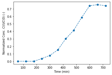
B. Plot normalized conc. as a function of time?
C. Find pore volume?
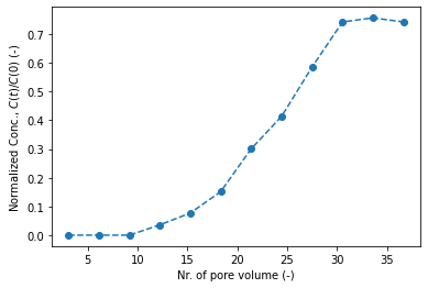
D. Plot normalized conc. as a function of pore volumes.
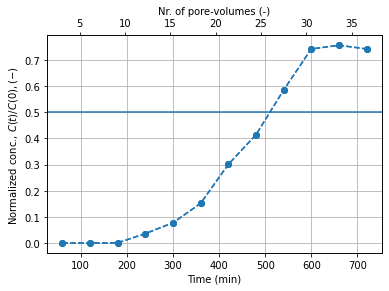
E. Find breakthrough time and number of flushing required to obtain a breakthrough concentration.
9.1.7. Solution Problem 21#
21. A & B
To normalize with initial concentration, we divide the outlet concentration with the initial concentration = 70 mg/L, we get:
#solution 21.A & B

c_ini = 70 # mg/L, initail concentration

c_n = c_mg/c_ini # (-), normalized concentration

d2 = {"Conc (mg/L)": c_mg, "Normalized Conc ()": c_n }
df2 = pd.DataFrame(d2)
 # display top 5 data

plt.plot(t_m, c_n, "--o",)
plt.xlabel("Time (min)"); plt.ylabel(r"Normalized Conc. $C(t)/C(0)$ (-)");

df2
| Conc (mg/L) | Normalized Conc () | |
|---|---|---|
| 0 | 0.00 | 0.000000 |
| 1 | 0.00 | 0.000000 |
| 2 | 0.00 | 0.000000 |
| 3 | 2.50 | 0.035714 |
| 4 | 5.40 | 0.077143 |
| 5 | 10.60 | 0.151429 |
| 6 | 21.05 | 0.300714 |
| 7 | 29.00 | 0.414286 |
| 8 | 41.00 | 0.585714 |
| 9 | 52.00 | 0.742857 |
| 10 | 53.00 | 0.757143 |
| 11 | 52.00 | 0.742857 |

Solution 21.C
A pore volume is the volume [L\(^3\)] of water that comes out of the saturated column. It can be obtained from the following equation:
Where, V = Volume of packing
To obtain a number of pore volume, use
where, \(V_x\) = Linear velocity [L/T], \(t\) = time [T], \(L\) = Column Length [L]
If volumetric flow (\(V_{vol}\)) is given, use
#solution 21.C
# Given

dia = 5 # cm, diameter of column
L_c = 1 # m, length of column
v_vol = 100 # mL/min, volumetric flow

#intermediate calculation
dia_m = dia/100 # m, diameter of column
v_c = np.pi/4*dia_m**2*L_c
v_volm = v_vol/10**6 # m³/min, vol. flow unit change

#compute and print
p_vol = np.round(v_volm*t_m/v_c,2) # (), nr. of pore volume, rounded to 2 decimal place

d3 = {"Time (min)":t_m, "Nr. of pore volumes ": p_vol}
df3 = pd.DataFrame(d3)

plt.plot(p_vol, c_n,"--o",)
plt.ylabel(r"Normalized Conc., $C(t)/C(0)$ (-)"); plt.xlabel("Nr. of pore volume (-)");

df3 # display top 5 data
| Time (min) | Nr. of pore volumes | |
|---|---|---|
| 0 | 60 | 3.06 |
| 1 | 120 | 6.11 |
| 2 | 180 | 9.17 |
| 3 | 240 | 12.22 |
| 4 | 300 | 15.28 |
| 5 | 360 | 18.33 |
| 6 | 420 | 21.39 |
| 7 | 480 | 24.45 |
| 8 | 540 | 27.50 |
| 9 | 600 | 30.56 |
| 10 | 660 | 33.61 |
| 11 | 720 | 36.67 |

Solution 21.E
fig = plt.figure()
ax1 = fig.add_subplot(111)
ax2 = ax1.twiny()

ax1.plot(t_m, c_n, "--o",)
ax1.yaxis.grid()
ax1.xaxis.grid()
ax1.set_xlabel("Time (min)")
ax1.set_ylabel(r"Normalized conc., $C(t)/C(0), (-)$ ")
ax2.plot(p_vol, c_n,"--o",)
ax2.set_xlabel("Nr. of pore-volumes (-)")
plt.axhline(y=.5)
<matplotlib.lines.Line2D at 0x2052d773a60>

Solution 21.E
The breakthrough is when outlet concentration is at 50% of the normalized concentration. In the figure the line is drawn. The breakthrough curve is then interpreted as:
After 510 minutes and 27 pore volumes of the input concentration the breakthrough concentration is obtained at the outlet
9.1.8. Homework Problem#
Homework Problem 11 - Conservative transport
rh11_1 = pn.pane.Markdown("""
NaCl is used to conduct a conservative tracer test in a Darcy column (length: 85 cm, diameter: 7.5 cm).
The volumetric flow rate is 10 mL/min and the NaCl is continuously injected (concentration: 55 mg/L).
The table shows NaCl concentrations measured at the column outlet at different times.

""",width = 600, style={'font-size': '12pt'})

rh11_2 = pn.pane.LaTeX(r"""
a) Normalise outlet concentration with injection concentration.<br>
b) Plot normalized concentration as a function of time.<br>
c) Determine graphically $t_{16}$, $t_{50}$, and $t_{84}$, where $t_x$ denotes the time when $x$% of the
injection concentration is reached at the column outlet.<br>
d) Determine effective porosity via $ n_e = \frac{Q\cdot t_{50}}{V}$ <br>
with $V$ = total volume of the column.<br>
e) Determine dispersivity via $\alpha = \frac{L}{8}\cdot \bigg(\frac{t_{84}-t_{16}}{t_{50}}\bigg)$

""",width = 600, style={'font-size': '12pt'})


dh11_t = np.array([15, 30, 45, 60, 75, 90, 105, 120, 135, 150, 165, 180])
dh11_C =  np.array([0, 0, 0, 2.5, 5.4, 10.6, 21.0, 29.1, 40.8, 51.7, 55.0, 55.0])

dh11 = {"Time [min]":dh11_t, "Conc. [mg/L]":dh11_C}

dfh11 = pd.DataFrame(dh11)

spacer = pn.Spacer(width=50)

rh11_3= pn.Column(rh11_1, rh11_2 )
pn.Row(rh11_3, spacer, dfh11)


