Reactive Mass Transport
Contents
2. Reactive Mass Transport#
(The contents presented in this section were re-developed principally by Dr. P. K. Yadav. The original contents are from Prof. Rudolf Liedl)
2.1. Motivation#
The last lecture dealt with the conservative transport processes and quantified the mass flow and flux emanating from those processes. The effects of these processes were evaluated as an isolated processes and as joint transport process.
Important conclusions from last lecture
\(J_{adv}>J_{dis}>>J_{diff}\) is observed in normal aquifers.
\(J_{diff}\) may only be useful as an individual processes in special aquifers, e.g., clayey aquifers.
In general aquifers, hydrodynamic dispersion \(J_{hyd} = J_{dis} + J_{diff}\) is used in the analysis of solute transport process.
Finally, the last chapter introduced Concentration Profile \((C-t)\) and Breakthrough Curve \((C-x)\) to visually evaluate solute transport in aquifers using Concentration \((C)\), a process output, as a function of time \((t)\) and space \((x)\).
This Lecture focuses on the reactive transport processes, which as already discussed involves the transport of solute with reaction processes. This course being an introductory groundwater course, sorption and degradation are the only two reaction types introduced and they are combined with the conservative transport processes- advection and dispersion. Eventully, the section evaluates the joint action of conservative transport and reactive processes limiting to 1-D scenario.
The lecture will, however, first deal with 3-D effects of dispersive process, which is more important to quantify the reactive processes.
2.2. Dispersive Mass Flow in 3-D#
In the last lecture we saw that concentration gradient \(\frac{\Delta C}{\Delta L}\) and flow velocity \(v\) drives dispersive and diffusive solute transport processes.
However, in the natural aquifers \(\frac{\Delta C}{\Delta L}\) is normally varying with space \((x,y,z)\) and time \((t)\). Therefore, a differential operator \(\big(\frac{\mathrm{d}}{\mathrm{d} x}\big)\) is more suitable representation of gradient than the difference operator \(\frac{\Delta C}{\Delta x}\). The differential operator also generalizes the gradient case.
Considering the differential operator, the diffusive mass flow and diffusive mass flux (= mass flow per unit area) in 1D is then expressed as:
and $\( j_{diff} = - n_e \cdot D_p \cdot \frac{\mathrm{d} C}{\mathrm{d}x} \)$
Likewise, the dispersive mass flow and dispersive mass flux (1-D) is:
The examples of these relations are presented in the last lecture Conservative Transport
2.3. 3-D concentration Gradient#
The concentration gradient \(\frac{\mathrm{d}C}{\mathrm{d}x}\) for 1-D solute transport problems is uni-directional, i.e, direction is fixed, and thus only the magnitude of the gradient is the important factor. However in higher dimensions, 2-D or 3-D, solute transport problems, the direction of gradient along with it’s magnitude in that direction has to be specified. Thus, for higher dimension solute transport problems, the concentration gradient becomes concentration vector, i.e., a quantity providing both magnitude and direction.
Thus, the representation of concentration gradient in Cartesian coordinate in 2-D and 3-D is:
and
The \(\nabla\), the inverted Delta symbol, is called the del or nabla operator. The vector grad \(C\) in the above relations points in the direction of the steepest increase of \(C\). However, for the Hydrogeologists, the concentration gradients as well the grad \(C\) points to the steepest decrease of \(C\).
2.4. Isotropic and Anisotropic Dispersion#
Corresponding the expression for the concentration gradient at higher dimensions, the expression for mass flow and flux becomes:
and the 3-D mass flux is:
The subscript in \({{disp, h}}\) refers to hydrodynamic dispersion which is sum of mechanical dispersion and diffusion. Likewise, the subscript \({{disp,\, hx}}\), \({{disp,\, hy}}\) and \({{disp,\, hz}}\) refers to dispersion components along the Cartesian coordinates. The corresponding mass flow and mass flux in the higher dimension is then:
and
The isotropic dispersion, rather an exceptional, the \(D_{hyd}\) in this case is:
where, \(D\) is direction independent dispersion coefficient and \(\alpha\) \([L]\) is dispersivity, which in:
heterogeneous aquifer: \(\alpha = \alpha(x,y,z)\) and in
homogeneous aquifer: \(\alpha = \text{constant}\)
For more practical cases and in normal aquifers, the 2-D and 3-D the dispersion for solute transport is direction dependent, i.e. anisotropic. Hence the \(D_{hyd}\) is not an scalar quantity but a matrix (tensor), which relates the concentration gradient (vector) to the dispersive mass flow (vector). However, if the princopal axes of the dispersion tensor \(D_{hyd}\) is made to coincide with the axes of a Cartesian coordinate system and the groundwater flow is considered uniform along the \(x-\)axis, the dispersive mass flux can be obtained from
with \(\alpha_L\), \(\alpha_{Th}\) and \(\alpha_{Tv}\) are longitudinal dispersivity, horizontal transverse dispversity and vertical transverse dispersivity, respectively. The statistical analysis of dispersivity data shows that \(\alpha_{L}>\alpha_{Th}>\alpha_{Tv}\) and the values differ roughly by an order of magnitude. This, however, is just a rule of thumb.
A quick example
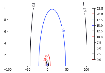
Discuss the role of 2D dispersitvity in column when discharge is limited at 10 m\(^3\)/d of a chemical with concentration 1 mg/L. The flow velocity can be assumed to be 0.05 m/d.
# Analytical solution from Bear (1976) - Line source, 1st-type input and infinte plane

# Input (values can be changed)
Co = 1 # mg/L, input concentration
Dx = 3 # m, Dispersion in x direction
Dy = Dx/10 # m
v = 0.05 # m/d
Q = 10 # m^3/d

## domain dimension and descritization (values can be changed)
xmin = -100; xmax= 101
ymin = 0.1; ymax = 11
[x, y] = np.meshgrid(np.linspace(xmin, xmax, 1000), np.linspace(ymin, ymax, 100)) # mesh

# Bear (1976) solution Implementation
#"k0: Modified Bessel function of second type and zero Order"

term1 = (Co*Q)/(2*np.pi* np.sqrt(Dx*Dy))
term2 = (x*v)/(2*Dx)
args = (v**2*x**2)/(4*Dx**2) + (v**2*y**2)/(4*Dx*Dy)
sol = term1*np.exp(term2)*sci.k0(args)

# plots
fig, ax = plt.subplots()
CS = ax.contour(x,y,sol, cmap='flag')
ax.clabel(CS, inline=1, fontsize= 10)
CB = fig.colorbar(CS, shrink=0.8, extend='both');
2.5. Equilibrium Sorption#
A reactive transport system can include a single reactive process, e.g., degradation, or combination of several multiple reactive processes, e.g. degradation and sorption. The inclusion of the reactive process(es) in the transport studies are site specific. The important to note is that an inclusion of a reactive process increases the complexity of transport problem.
In this course we limit ourselves with the following two types of reaction processes:
1. Sorption
2. Degradation
Acid-base reaction, precipitation-dissolution reaction, organic combustion etc. are among the reactions type that can be part of the reactive process individually or in any combination.
Also an important distinction is the rate or speed of the reaction. One distinguishes between time-dependent reaction (kinetics) or time-independent reactions (steady-state or equilibrium). Special reaction rates such as instantaneous reaction (extremely fast reaction) can also be part of the reaction process in the transport system.
2.6. Sorption Basics#
Sorption is a rather a general term used to indicate both adsorption and absorption. But in this course the sorption refers to only adsorption.
Adsorption can be more formally defined as the process of accumulation of dissolved chemicals on the surface of a solid, e.g., accumulation of a chemicals dissolved in groundwater on the surface of the aquifer material.
The figure below clarifies the adsorption process.
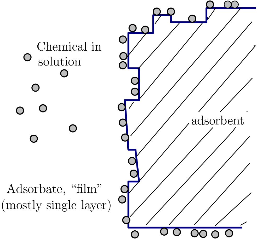
Fig. 2.1 Sorption terminology#
In the figure chemical in solution (the circular objects) more often called solute in the water is found to attach is the solid surface. The figure presents the following two important terms part of the adsorption process:
Adsorbent: The solid onto which the chemicals are attached. More formally, adsorbents provide adsorption sites for solutes.
Adsorbate: These are solutes that are attached on the adsorbent.
Based on the figure, adsorption can be considered as a partition process that divides the chemical originally present in water between adsorbent and water.
Quite often adsorption is a reversible process, i.e., adsorbed chemicals can get back to water phase. This process is called desorption.
Speaking about equilibrium, this is reached when
adsorption rate \(\rightleftharpoons \) desorption rate
Adsorption in groundwater is often a rapid process. Although sorption kinetics can be important, the description in this introductory level course is limited to equilibrium sorption. Thus, we learn next to quantify equilibrium sorption.
2.7. Adsorption Isotherms#
The adsorption process that has reached equilibrium can be relatively easily quantified with the use of empirical models called isotherms. These models are often simple algebraic equation that relates solute concentrations partitioned between the adsorbate and adsorbent at constant temperature. More than 15 different isotherm models can be found in the literature. However, in groundwater reactive transport studies the following three are the two most commonly used isotherms:
Henry or Linear isotherm
Freundlich isotherm
For quantification, laboratory based experiments are performed using solids from subsurface and chemicals of interest. The laboratory observations are then graphically fitted with empirical isotherm models to quantify adsorption properties. Figure below shows isotherms that are particularly observed in groundwater transport studies. As can be observed in the figure sorption coefficient (\(K\)) is the common quantities obtained from isotherm models.
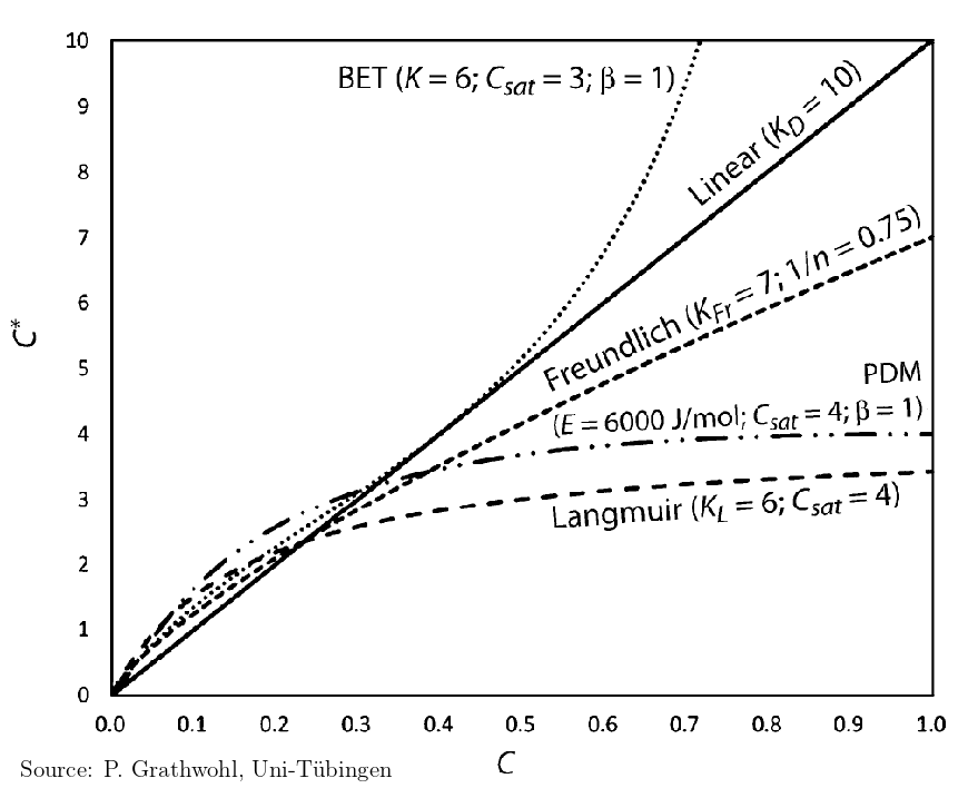
Fig. 2.2 Different types of sorption isotherms#
2.8. Henry Isotherm#
The Henry isotherm (Henry, 1803) is based on the idea of a linear relationship between the solute concentration \(C\) and the adsorbate:adsorbent mass ratio \(C_a\). Henry isotherm is quite often also called linear isotherm or the \(K_d\) model. Mathematically, the Henry isotherm is:
with
\(C\) = solute concentration [ML\(^{-3}\)]
\(C_a\) = mass ratio adsorbate:adsorbent [M:M]
\(K_d\) = distribution or partitioning coefficient [L\(^3\)M\(^{-1}\)].
Often symbols \(C_s\) or \(s\) are used instead of \(C_a\).
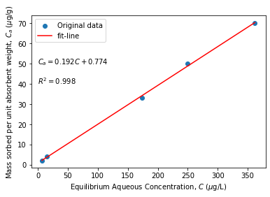
The Henry model has been most widely used in groundwater transport studies. This is largely because of the simplicity (see equation) of the model and it’s applicability in representing adsorption process more generally observed in groundwater studies. \(K_d\), the partitioning coefficient, is particularly used in groundwater transport studies. It is equal to the slope of the Henry isotherm.
A quick example
From the experimental data provided below, obtain the Henry distribution coefficient.
# Example of Henry isotherm (Source: Fetter et al. 2018)

# Following sorption data are available:

C = np.array([7, 15, 174, 249, 362]) # ug/L, Eq. concentration
Ca = np.array([2, 4, 33, 50, 70]) # ug/g, Eq. sorbed mass

# linear- fit y = m*x+c

slope, intercept, r_value, p_value, std_err = stats.linregress(C, Ca)
print("slope = %0.3f    intercept= %0.3f  R-squared=%0.4f" % (slope, intercept, r_value**2),'\n')
fit_line = slope*C + intercept

#plot

plt.scatter(C, Ca, label= "Original data") # data plot
plt.plot(C, fit_line, color = "red", label = "fit-line")
plt.legend(); plt.xlabel(r"Equilibrium Aqueous Concentration, $C$ ($\mu$g/L) ")
plt.ylabel(r"Mass sorbed per unit absorbent weight, $C_a$ ($\mu$g/g) ");
plt.text(0, 50, '$C_a=%0.5s C + %0.5s$'%(slope, intercept), fontsize=10)
plt.text(0, 40, '$R^2=%0.5s $'%(r_value**2), fontsize=10)

# Output

print("The required partition coefficient = slope,= %0.5s L/g " % slope)
slope = 0.192    intercept= 0.775  R-squared=0.9990

The required partition coefficient = slope,= 0.192 L/g
2.9. Freundlich Isotherm#
Freundlich isotherm (Freundlich, 1907) is a more general isotherm. It is based on the idea of a power law, i.e., includes also the non-linear behaviour, relating the solute concentration \(C\) to the adsorbate:adsorbent mass ration \(C_a\). The isotherm is mathematically given as
with
\(C\) = solute concentration [ML\(^{-3}\)]
\(C_a\) = mass ratio adsorbate:adsorbent [M:M]
\(n\) = Freundlich exponent [-]
\(K_{Fr}\) = Freundlich partitioning coefficient [(M:M)/(M/L\(^3)^n\)].
The Freundlich isotherm equation can be easily linearized by applying logarithmic transformation of the equation, which gives
\begin{eqnarray*} \log C_a = \log K_{Fr} + n\cdot \log C \end{eqnarray*}
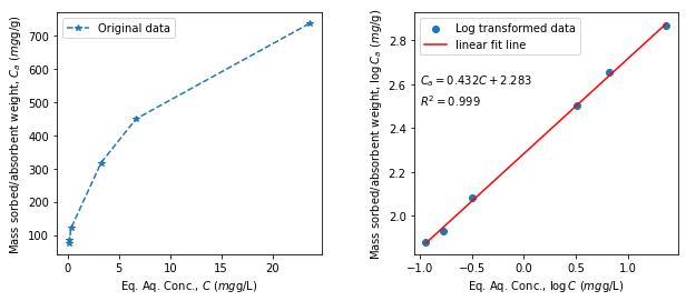
The above equation resembles the straight line equation \(y = b + a \cdot x b\), in which \(b\equiv \log K_{Fr}\) is the intercept and \(a\equiv n\) the slope. Thus, from fitting the adsoprtion experimental results with the above equation, both \(n\) and \(K_{Fr}\) can be obtained.
A quick example
From the experimental data provided below, obtain the Freundlich partitioning coefficient and Freundlich exponent.
# Example of Freundlich isotherm

# Following sorption data are available:

Cf= np.array([23.6, 6.67, 3.26, 0.322, 0.169, 0.114]) # mg/L, Eq. concentration
Caf = np.array([737, 450, 318, 121, 85.2, 75.8]) # mg/g, Eq. sorbed mass

logCf = np.log10(Cf) # log10 transformation of data
logCaf = np.log10(Caf)

# fitting: y = mx +c
slope, intercept, r_value, p_value, std_err = stats.linregress(logCf, logCaf)
print("slope: %0.3f    intercept: %0.3f  R-squared: %0.3f" % (slope, intercept, r_value**2))
fit_line = slope*logCf + intercept

# plots
plt.figure(figsize=(10,4))

plt.subplot(121)
plt.plot(Cf, Caf, "*--", label= "Original data")
plt.legend(); plt.xlabel(r"Eq. Aq. Conc., $C$ ($mg$g/L) ");
plt.ylabel(r"Mass sorbed/absorbent weight, $C_a$ ($mg$g/g) ");

plt.subplot(122)
plt.scatter(logCf, logCaf, label="Log transformed data")
plt.plot(logCf, fit_line, color="red", label= "linear fit line")
plt.legend(); plt.xlabel(r"Eq. Aq. Conc., $\log C$ ($mg$g/L) ");
plt.ylabel(r"Mass sorbed/absorbent weight, $\log C_a$ ($mg$/g) ");
plt.text(-1, 2.6, '$C_a=%0.5s C + %0.5s$'%(slope, intercept), fontsize=10)
plt.text(-1, 2.5, '$R^2=%0.5s $'%(r_value**2), fontsize=10)
plt.subplots_adjust(wspace=0.35)

print("Freundlich partitioning coefficient =  %0.5s (mg/g)1/n (mg/L) and  Freundlich exponent = %0.4s"  % (10**intercept, slope))
slope: 0.433    intercept: 2.283  R-squared: 0.999
Freundlich partitioning coefficient =  191.8 (mg/g)1/n (mg/L) and  Freundlich exponent = 0.43
2.10. Retardation Factor (for Henry Isotherm)#
The net effect of adsorption is the retarded movement of solute in comparison to the average flow of the groundwater. The term Retardation Factor \((R)\) is defined that quantifies the retarded movement of solute. The formulation of \(R\) is based on the type of isotherm. For Henry isotherm \(R\) can be straightforwardly calculated with the help of a mass budget.
For this purpose, an aquifer volume \(V\) with the effective porosity \(n_e\) is considered (see fig. below)
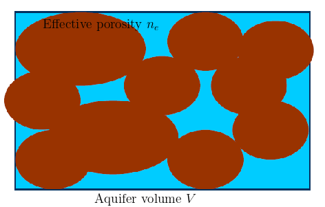
Fig. 2.3 Retardation factor#
The steps involved are:
Total volume: \(V\)
Water volume: \(n_e \cdot V\)
Mass of dissolved chemical: \(n_e \cdot V \cdot C\)
Volume of solid: \((1-n_e)\cdot V\)
Density of solid material: \(\rho\)
Mass of solid: \(\rho \cdot(1-n_e)\cdot V\)
Mass of adsorbate: \(\rho \cdot(1-n_e)\cdot V\cdot C_a\) = \((1-n_e)\cdot\rho \cdot V \cdot K_d \cdot C\)
Total mass: \(n_e\cdot V \cdot C + (1-n_e)\cdot\rho \cdot V\cdot K_d \cdot C = n_e \cdot R \cdot V \cdot C\)
with Retardation factor $\(R = 1 + \frac{1-n_e}{n_e}\cdot \rho \cdot K_d\)$
The expression for \(R\) can be further modified by using bulk density \(\rho_b\) \(= (1-n_e)\cdot \rho\) = mass of solid/total volume. This leads to
As can be observed from the equation, \(R = 1\) when there is no adsorption, i.e., when \(K_d= 0\).
A quick example
Calculate the retardation factor from the provided data.
print("\033[0m You can change the provided values.\n")

ne = 0.4 #effective porosity [-]
rho = 1.25 # density of solid material [kg/m³]
Kd = 0.2 # distribution or partition coefficient [m³/kg]

#intermediate calculation
rho_b = (1-ne)*rho

#solution
R=1+(rho_b/ne)*Kd

print("effective porosity = {}\ndensity of solid material = {} kg/m³\nDistribution or partition coefficient = {} m³/kg\n".format(ne, rho, Kd))
print("\033[1mSolution:\033[0m\nThe resulting retardation factor is \033[1m{:02.4}\033[0m.".format(R))
 You can change the provided values.

effective porosity = 0.4
density of solid material = 1.25 kg/m³
Distribution or partition coefficient = 0.2 m³/kg

Solution:
The resulting retardation factor is 1.375.
2.11. Degradation#
Degradation leads to alteration or transformation of chemical structure of chemicals. This contrasts to adsorption in which chemical structure is not altered. In adsorption (or desorption) the original chemical is partitioned between the solid particles and water. It is degradation that eventually lead to removal of the original chemical from the groundwater. The transformation of original chemical, due to degradation, results to so-called daughter products (metabolites). The new chemical(s) can make groundwater more suitable (decrease contamination) or further contaminate it.
In groundwater studies, degradation can appear as:
Radioactive decay
Microbial degradation (bio-degradation)
Chemical degradation
There are several approaches to quantify degradation process. A common aspect to most of them is the assumption of time-dependency (or Kinetics ).
2.12. \(n^{th}\) - Order Degradation Kinetics#
The general equation for the degradation kinetics is:
with \(t\) = time [t]
\(C\) = solute concentration [ML\(^{-3}\)]
\(n\) = order of the degradation kinetics [ - ] (\(n\geq 0)\)
\(\lambda\) = degradation rate constant [(ML\(^{-3})^{(1-n)}\)T\(^{-1}\)].
Considering the initial concentration (or input concentration) \(C_0\), the solutions of the kinetics equation are:
and
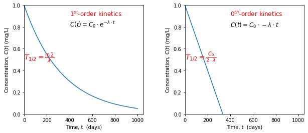
The half life \((T_{1/2})\), which is the time span elapsing until the initial concentration \(C_0\) is reduced by half, is an important time-scale in the degradation analysis. \(T_{1/2}\) is \(C_0\) dependent in nearly all cases with an exception for 1\(^\text{st}\)- order degradation kinetics. 0\(^{th}\)-order and the 1\(^\text{st}\)- order degradation kinetics are most commonly observed in groundwater studies. The \((T_{1/2})\) of these orders are:
As can be observed above \(T_{1/2}\) is independent of concentration for the 1\(^{\text{st}}\)-order degradation kinetics.
Another important properties of the degradation kinetics is that for \(n\geq 1\) the solute concentration asymptotically approaches zero, whereas for \(n<1\), the solute concentration actually reaches zero
# behaviour of degradation kinetics

#input - you may change the values
Co = 1 # mg/L, initial concentration
la = 0.003 # unit is order dependent. For n=1, 1/t

# main equation
Z_order = lambda t: Co* np.exp(-la*t) # for n = 0
F_order = lambda t: Co-la*t # for n = 1

# simulation for t
t = np.linspace(1,1000, 1000) # 1000 time units
Z_results = Z_order(t)
F_results = F_order(t)

# plots
plt.figure(figsize=(10,4))

# n = 1
plt.subplot(121)
plt.plot(t, Z_results)
plt.ylim(0, Co); plt.xlim(0)
plt.text(400, Co*0.8, r"$C(t) = C_0 \cdot e^{-\lambda \cdot t} $", fontsize = 12)
plt.text (400, Co*0.9, r"1$^{st}$-order kinetics", color = "red", fontsize = 12)
plt.text(0, Co/2, r"$T_{1/2}= \frac{\ln 2}{\lambda}$", color= "red", fontsize=14)
plt.xlabel("Time, t  (days)"); plt.ylabel(r"Concentration, $C(t)$ (mg/L)")

# n = 0
plt.subplot(122)
plt.plot(t, F_results)
plt.ylim(0, Co); plt.xlim(0)
plt.text(400, Co*0.8, r"$C(t) = C_0 \cdot-\lambda \cdot t} $", fontsize = 12)
plt.text (400, Co*0.9, r"0$^{th}$-order kinetics", color = "red", fontsize = 12)
plt.text(0, Co/2, r"$T_{1/2}= \frac{C_0}{2\cdot \lambda}$", color= "red", fontsize=14)
plt.xlabel("Time, t  (days)"); plt.ylabel(r"Concentration, $C(t)$ (mg/L)")

plt.subplots_adjust(wspace=0.35)
2.13. Radioactive decay#
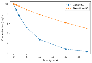
Radioactive decay is degradation of a chemical due to radiation. The radioactive decay is limited to radioactive chemicals such as Cobalt, Cesium, Iodine. This decay obeys the 1\(^\text{st}\)- order degradation kinetics and therefore the half-life is \(T_{1/2} = \frac{\ln 2}{\lambda}\). \(T_{1/2}\) is characteristic property of radioactive chemicals and it can be used to compute degradation rate (\(\lambda\)).
# Example of Radioactive decaly

#experimental results

t = [0, 1, 2, 5, 10, 20, 28 ] # yr, time
Co_60 = [10, 8.76, 7.68, 5.17, 2.68, 0.72, 0.25] # mg/L, Cobalt 60 conc.
So_90 = [10, 9.76, 9.52, 8.84, 7.81, 6.10, 5] # mg/L, Strontium 90 Conc.

z_list = list(zip(t, Co_60, So_90))

Cols= ["time (a)", "Cobalt 60 (mg/L)", "Strontium 90 (mg/L)"]
df = pd.DataFrame(z_list, columns=Cols)
print(df)

# computing
TH_Co60 = 28 # yr, Half life of Cobalt 60
TH_St90 = 5.26 # yr, Half life of Strontium 90
la_Co60 = np.log(2)/TH_Co60 # 1/yr, degradation rate of Cobalt 60
la_St90 = np.log(2)/TH_St90 # 1/yr, degradation rate of Strontium 90

# visualize
plt.plot(t, Co_60, "o--", label = "Cobalt 60")
plt.plot(t, So_90, "v--", label= "Strontium 90")
plt.xlabel("Time (years)"); plt.ylabel("Concentration (mg/L)")
plt.legend();

print("\n The degradation rate (\u03BB) for Cobalt 60 = %0.5s 1/y and for Strontium 90 = %0.5s 1/y \n"  % (la_Co60, la_St90))
   time (a)  Cobalt 60 (mg/L)  Strontium 90 (mg/L)
0         0             10.00                10.00
1         1              8.76                 9.76
2         2              7.68                 9.52
3         5              5.17                 8.84
4        10              2.68                 7.81
5        20              0.72                 6.10
6        28              0.25                 5.00

 The degradation rate (λ) for Cobalt 60 = 0.024 1/y and for Strontium 90 = 0.131 1/y
2.14. Joint Action of Conservative and Reactive Transport (1D)#
2.15. Concentration Profile#
Figure below presents the joint action of conservative transport with equilibrium sorption (linear isotherm) and degradation. The figure shows the solute concentration \(C\) (in water) at the same time-levels for various combinations of acting processes.
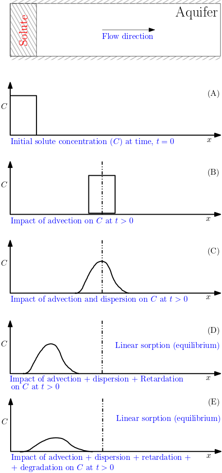
Fig. 2.4 1D Conservative and Reactive Transport#
The figure can be explained in the following way:
(A): The solute is initially present at constant concentration in a limited area.
(B): Solute spreads only due to advection. Due to absence of dispersion there is no (1D) spreading effect.
(C): Inclusion of dispersion process causes spread of concentration. As retardation is absence the front centreline remains unchanged
(D): The inclusion of retardation (\(R\)) with advection and dispersion leads to removal of chemicals from water and as well the retarded movement of the chemical front.
(E): The inclusion of retardation along with degradation and conservative transport process leads to high removal of chemical from water.
2.16. Breakthrough Curve#
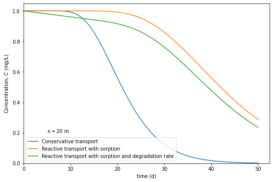
Breakthrough curves provide a time-dependent spread of chemicals in the groundwater. The inclusion of multiple processes are normally solved using numerical models. Analytical models are available for limited processes and simplified problems. A 1-D analytical solution by Kinzelbach (1987) provide a transient (time-dependent) solution of reactive transport problem with inclusion of equilibrium linear sorption represented by retardation \((R)\), first-order degradation rate \((\lambda)\) and the conservative transport quantities - dispersion \((D)\) and advection. The solution is given as:
with \(C_0\) = input/source concentration [ML\(^{-3}\)]
\(t\) = time [T]
\(v\) = groundwater flow velocity [LT\(^{-1}\)]
erfc() = represents the complementary error function See here for details. erfc() can be easily computed using Python Scipy special function library.
# Breakthrough curve using Kinzelbach (1987) analytical solution Main function

# The main function - you may change the value of C_o, lam, R, Dx, v, x
# C_o = input concentration, mg/L
# lam = 0 # 1/d, degradation rate, 1/d
# R = retardation factor, ()
# Dx = dispersion coeff. along x, m^2/d
# v = groundwater velocity, m/d
# x = position where C is to be measured, m

def Cx(t, C_o= 1, lam = 0, R=1, Dx=1, v= 10, x = 20):
    sterm = C_o*np.exp(-lam*t)
    erf_ag1 = (R*x-v*t)/(2*np.sqrt(Dx*R*t))
    erf_ag2 = (R*x+v*t)/(2*np.sqrt(Dx*R*t))

    C = sterm*(1-(0.5*sci.erfc(erf_ag1)-0.5*np.exp((v*x)/Dx)*sci.erfc(erf_ag2)))
    return C
# Computing Case 1: Conservative process- R = 1, Lambda = 0
t1 = np.linspace(1e-5,50,1000) # times, d
C1 = Cx(t1, C_o= 1, lam = 0, R=1, Dx=1, v= 1, x = 20)

# Computing Case 2: Conservative system + Retardation - R = 2, Lambda = 0
t2 = np.linspace(1e-5,50,1000) # times, d
C2 = Cx(t2, C_o= 1, lam = 0, R=2, Dx=1, v= 1, x = 20)

# Computing Case 3: Conservative system + Retardation + degradation - R = 2, Lambda = 0.004
t3 = np.linspace(1e-5,50,1000) # times, d
C3 = Cx(t3, C_o= 1, lam = 0.004, R=2, Dx=1, v= 1, x = 20)

# plots - this should be adjusted as required

plt.figure(figsize=(9, 6))

plt.plot(t1, C1, label="Conservative transport")
plt.plot(t2, C2, label = "Reactive transport with sorption")
plt.plot(t3, C3, label = "Reactive transport with sorption and degradation rate")
plt.legend(loc= 3); plt.xlim(0), plt.ylim(0)
plt.xlabel("time (d)"); plt.ylabel(r"Concentration, $C$ (mg/L)")
plt.text(5, 0.2, r"$x= 20$ m")
Text(5, 0.2, '$x= 20$ m')
2.17. Mass (Re-)Distribution During Injection / Extraction#
Consider a scenario:
Water is injected into a certain portion of an aquifer with total volume \(V\), bulk density \(\rho_b\) and effective porosity \(n_e\). Assume that the injected water contains a chemical of total mass \(M\), which is adsorbed by the aquifer materials under equilibrium conditions according to Henry isotherm (quantified by \(K_d\)$).
Bases on the assumption of sorption equilibrium, the total mass \(M\) of the chemical is instantaneously(!) split up into a dissolved and a sorbed part. In such case, the mass distribution can be computed as follows (with \(R\) = retardation factor, \(\rho_b\) = bulk density):
\begin{align} M &= n_e \cdot V \cdot C + V\cdot\rho_b \cdot C_a \ &= n_e \cdot V \cdot C + V \cdot \rho_b \cdot K_d \cdot C\ &= n_e \cdot (1 + \rho_b \cdot K_d/n_e) \cdot V \cdot C\ &= n_e \cdot R \cdot V \cdot C \end{align}
In which,
\(n_e \cdot V \cdot C\) = dissolved mass
\(V\cdot\rho_b \cdot C_a\) = mass of adsorbate
For the dissolved mass we thus have \(n_e \cdot V \cdot C = M/R\) and consequently the mass of adsorbate is:
\(V\cdot\rho_b \cdot C_a = M- M/R = (1-1/R)\cdot M\)
The same approach can be adopted for the extraction scenarios, i.e. equilibrium desorption.
2.18. Additional Tool#
The additional tool: 1D-Advection-Dispersion Simulation Tool simulates all the concepts that are provided above. The tool simulates:
1D solute transport in porous media (e.g., laboratory column)
uses unifrom cross-section
steady-state water flow
input of tracer
The output are then:
spreading of tracer due to advection and mechanical dispersion
computation and graphical representation of a breakthrough curve
comparison with measured data.
